Using Prior Information as Restrictions

This tutorial demonstrates how to incorporate prior information about unit similarities using the unrestricted/restricted unit functionality of OptimalUnitAveraging — the large-N regime.

By the end, you should be able to:

1. Understand the motivation for restricted/unrestricted unit classification.

2. Specify unrestricted/restricted unit restrictions in OptimalUnitAverager.

3. Interpret the resulting weight distributions.

Functionality covered

OptimalUnitAverager: using the unrestricted_unit_bool argument for the large-N regime.

import numpy as np
import pandas as pd
from docs_utils import plot_germany, prepare_frankfurt_example

from unit_averaging import IndividualUnitAverager, OptimalUnitAverager

Following along

If you would like to follow along on a local machine, please download the contents of the data folder here . To recreate the plots, also download the docs_utils.py file .

Some Background

In our first application of OptimalUnitAverager in Getting Started, the weight of every unit could be determined separately. This is a flexible approach that allows the averager to choose which units are important without requiring prior information on unit similarities from the user.

However, when dealing with many units, this approach may have two key drawbacks:

• It may overfit: May assign non-zero weights to irrelevant units.

• It ignores known similarities between units.

OptimalUnitAverager supports an approach that can reduce the dimensionality of the averaging problem by grouping units into two categories:

• “Unrestricted” units: units whose weights are still chosen freely (and may be chosen to zero).

• “Restricted” units: the weights of all the restricted units are equal. The algorithm only chooses how much weight overall to give to the average of restricted units.

Using restricted units is called the “large-N” regime for theoretical reasons (see the original paper), in contrast to the “fixed-N” regime with no restricted units. The large-N names comes from the fact that the approach is more effective and theoretically justified when the set of restricted units is large.

In practice, the choice of unrestricted vs. restricted units reflects prior information: units that may be more important for prediction (more similar, have tighter economic links, etc.) should be left unrestricted. All other units should be restricted.

At the same time, it’s important to highlight the following point:

Choice of unrestricted units is a tuning parameter

The choice of unrestricted units is not a causal statement about the underlying reality. OptimalUnitAverager will optimally adapt to the specified structure to the extent possible.

Restricted and Unrestricted Units in Practice

We now apply this large-N approach in a worked example. We revisit the Frankfurt unemployment forecasting example from Getting Started, now incorporating prior information about regional similarities. Again, the task is to predict the change in unemployment in Frankfurt in January 2020 from a panel of 150 German labor market districts, Frankfurt included.

We load our prepared individual estimates, individual covariance matrices, and the focus function for forecasting the target unemployment rate:

ind_estimates, ind_covar_ests, forecast_frankfurt_jan_2020 = prepare_frankfurt_example()

/home/runner/work/unit-averaging/unit-averaging/docs/examples/docs_utils.py:109: PerformanceWarning: DataFrame is highly fragmented.  This is usually the result of calling `frame.insert` many times, which has poor performance.  Consider joining all columns at once using pd.concat(axis=1) instead. To get a de-fragmented frame, use `newframe = frame.copy()`
  german_data["Germany_lag"] = german_data["Deutschland"].shift(1)

Specifying Unit Restrictions

We assume Hessen regions (Frankfurt’s state) are potentially relevant for forecasting Frankfurt’s unemployment, with Frankfurt influenced by the regions in its state. These become unrestricted units while all others are restricted.

It is important to stress that this choice means the algorithm is free to choose any weight for regions in Hessen (including zero). This flexibility allows the averager to make use of more relevant unrestricted units and to discard the less relevant ones.

Specifically, the regions in Hessen are:

hessen_regions = [
    "Kassel",
    "Korbach",
    "Bad Hersfeld - Fulda",
    "Marburg",
    "Limburg - Wetzlar",
    "Gießen",
    "Hanau",
    "Wiesbaden",
    "Bad Homburg",
    "Frankfurt",
    "Offenbach",
    "Darmstadt",
]

Information about whether a unit is unrestricted is boolean, with True meaning that a unit is unrestricted, and False that it is restricted.

unrestricted_units = {region: (region in hessen_regions) for region in ind_covar_ests}

print(unrestricted_units)

{'Aachen - Düren': False, 'Aalen': False, 'Ahlen - Münster': False, 'Annaberg-Buchholz': False, 'Ansbach - Weißenburg': False, 'Aschaffenburg': False, 'Augsburg': False, 'Bad Homburg': True, 'Bad Kreuznach': False, 'Bad Oldesloe': False, 'Balingen': False, 'Bamberg - Coburg': False, 'Bautzen': False, 'Bayreuth - Hof': False, 'Bergisch Gladbach': False, 'Bad Hersfeld - Fulda': True, 'Berlin Mitte': False, 'Berlin Nord': False, 'Bielefeld': False, 'Bochum': False, 'Bonn': False, 'Braunschweig - Goslar': False, 'Bremen - Bremerhaven': False, 'Brühl': False, 'Berlin Süd': False, 'Celle': False, 'Chemnitz': False, 'Cottbus': False, 'Darmstadt': True, 'Deggendorf': False, 'Detmold': False, 'Donauwörth': False, 'Dortmund': False, 'Dresden': False, 'Duisburg': False, 'Düsseldorf': False, 'Eberswalde': False, 'Elmshorn': False, 'Coesfeld': False, 'Emden - Leer': False, 'Essen': False, 'Frankfurt': True, 'Frankfurt (Oder)': False, 'Freiberg': False, 'Freiburg': False, 'Freising': False, 'Fürth': False, 'Gelsenkirchen': False, 'Gießen': True, 'Göppingen': False, 'Göttingen': False, 'Greifswald': False, 'Flensburg': False, 'Hamburg': False, 'Hameln': False, 'Hamm': False, 'Hanau': True, 'Hannover': False, 'Heide': False, 'Heidelberg': False, 'Heilbronn': False, 'Helmstedt': False, 'Herford': False, 'Hildesheim': False, 'Hagen': False, 'Ingolstadt': False, 'Iserlohn': False, 'Kaiserslautern - Pirmasens': False, 'Karlsruhe - Rastatt': False, 'Kassel': True, 'Kempten - Memmingen': False, 'Kiel': False, 'Koblenz - Mayen': False, 'Köln': False, 'Konstanz - Ravensburg': False, 'Korbach': True, 'Krefeld': False, 'Landau': False, 'Landshut - Pfarrkirchen': False, 'Leipzig': False, 'Limburg - Wetzlar': True, 'Ludwigshafen': False, 'Lüneburg - Uelzen': False, 'Lörrach': False, 'Lübeck': False, 'Ludwigsburg': False, 'Mainz': False, 'Mannheim': False, 'Marburg': True, 'Meschede - Soest': False, 'Mettmann': False, 'Mönchengladbach': False, 'Montabaur': False, 'München': False, 'Nagold - Pforzheim': False, 'Neubrandenburg': False, 'Neumünster': False, 'Neuruppin': False, 'Neuwied': False, 'Nienburg - Verden': False, 'Nordhorn': False, 'Nürnberg': False, 'Offenburg': False, 'Oldenburg - Wilhelmshaven': False, 'Oschatz': False, 'Osnabrück': False, 'Oberhausen': False, 'Offenbach': True, 'Paderborn': False, 'Passau': False, 'Pirna': False, 'Plauen': False, 'Potsdam': False, 'Recklinghausen': False, 'Riesa': False, 'Rosenheim': False, 'Regensburg': False, 'Rostock': False, 'Rottweil - Villingen-Schwenningen': False, 'Reutlingen': False, 'Rheine': False, 'Saarland': False, 'Sachsen-Anhalt Nord': False, 'Schwäbisch Hall - Tauberbischofsheim': False, 'Schwandorf': False, 'Schweinfurt': False, 'Schwerin': False, 'Siegen': False, 'Solingen - Wuppertal': False, 'Sachsen-Anhalt Ost': False, 'Stade': False, 'Stralsund': False, 'Stuttgart': False, 'Sachsen-Anhalt Süd': False, 'Sachsen-Anhalt West': False, 'Thüringen Mitte': False, 'Thüringen Nord': False, 'Thüringen Ost': False, 'Thüringen Südwest': False, 'Traunstein': False, 'Trier': False, 'Ulm': False, 'Weilheim': False, 'Wesel': False, 'Wiesbaden': True, 'Vechta': False, 'Würzburg': False, 'Zwickau': False, 'Waiblingen': False, 'Weiden': False, 'Deutschland': False}

Since our ind_estimates and ind_covar_ests are dictionaries indexed by regions, the information on unrestricted units should also be a dictionary indexed by the same regions. Otherwise the averager would not be able to match the information on unrestricted units to the units themselves.

Fitting the Averager

With the information on unrestricted units specified, we can now create an instance of OptimalUnitAverager with these unit restrictions.

We pass unrestricted_units to the unrestricted_units_bool argument of the averager:

averager = OptimalUnitAverager(
    focus_function=forecast_frankfurt_jan_2020,
    ind_estimates=ind_estimates,
    ind_covar_ests=ind_covar_ests,
    unrestricted_units_bool=unrestricted_units,
)

We can now fit our averager and examine the predicted value:

averager.fit(target_id="Frankfurt")
print(averager.estimate.round(3))

-0.112

The predicted value is quite close to the individual-specific estimate:

ind_averager = IndividualUnitAverager(
    focus_function=forecast_frankfurt_jan_2020,
    ind_estimates=ind_estimates,
)
ind_averager.fit(target_id="Frankfurt")
print(ind_averager.estimate.round(3))

-0.115

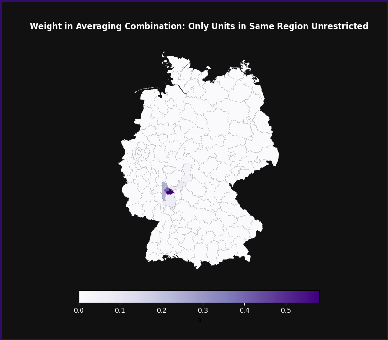
Finally, we can examine the fitted weights. First, we plot them:

weight_df = pd.DataFrame({"aab": averager.keys, "weights": averager.weights})
# sphinx_gallery_thumbnail_number = 1
fig, ax = plot_germany(
    weight_df,
    "Weight in Averaging Combination: Only Units in Same Region Unrestricted",
    cmap="Purples",
    vmin=-0.005,
    vmax=0.3,
)

We can take a deeper look at the weights of the restricted and the unrestricted units by accessing the weights attribute of the averager.

We first look at the total weight received by the set of restricted units. This total is what is chosen by the averager. Then this total is equally divided between the restricted units. In our case, we have:

sum(averager.weights[~np.isin(averager.keys, hessen_regions)]).round(3)

np.float64(0.0)

Even as a group, the restricted units receive effectively no weight. This means the model relies almost entirely on the unrestricted Hessen regions for forecasting Frankfurt’s unemployment.

For the regions in Hessen, the weights can vary freely, and we examine them individually:

print(
    pd.Series(
        {
            reg: weight.round(3)
            for reg, weight in zip(
                averager.keys[np.isin(averager.keys, hessen_regions)],
                averager.weights[np.isin(averager.keys, hessen_regions)],
                strict=True,
            )
        }
    )
)

Bad Hersfeld - Fulda    0.018
Bad Homburg             0.121
Darmstadt               0.035
Frankfurt               0.207
Gießen                  0.000
Hanau                   0.038
Kassel                  0.000
Korbach                 0.000
Limburg - Wetzlar       0.000
Marburg                 0.000
Offenbach               0.581
Wiesbaden               0.000
dtype: float64

The averager assigns almost all weights to Frankfurt itself, and two bordering regions — Offenbach and Bad Homburg. In other words, even within Hessen, the averager concentrates weight on the metropolitan region of Frankfurt.

At the same time, there is some variation in the weights. This suggests that the averaging prediction likely has lower variance than the individual-specific prediction.

Stein unit averaging

For cases where you want to restrict all non-target units (Stein-like shrinkage), SteinUnitAverager offers a convenient interface. There is no need to specify unrestricted units when using SteinUnitAverager.