Getting Started with Optimal Unit Averaging

This tutorial walks you through the complete workflow of unit_averaging. It lays out a template for going from raw data to optimal estimation with unit averaging. Throughout, we use a real-world example: forecasting Frankfurt’s unemployment rate using data from 150 German regions, while taking into account the differences in regional dynamics.

By the end, you should be able to:

1. Define a focus function to map model parameters to your target (e.g., a forecast),

2. Prepare data on unit-level estimates.

3. Define and fit an optimal unit averager.

4. Compare results against the baseline of no averaging.

Functionality covered

OptimalUnitAverager, IndividualUnitAverager, and InlineFocusFunction

import numpy as np
import pandas as pd
from docs_utils import plot_germany
from statsmodels.tsa.ar_model import AutoReg

from unit_averaging import (
    IndividualUnitAverager,
    InlineFocusFunction,
    OptimalUnitAverager,
)

Following along

If you would like to follow along on a local machine, please download the contents of the data folder here . To recreate the plots, also download the docs_utils.py file .

Problem, Key Idea, Data

Introduction

Suppose that it is December, 2019 and we want to optimally forecast the change in the unemployment rate in Frankfurt in the next month. At our disposal we have a panel (longitudinal) dataset of unemployment rates for all the regions of Germany, Frankfurt included.

What is the key challenge to using all this data efficiently? The regions are different in unseen ways (or heterogeneous): each of them has its own unemployment dynamics, driven by differences in their economies, populations, and laws. Throwing the data on all the regions into a single prediction model usually may yield a very biased forecast for Frankfurt (or for any other specific region).

Unit averaging is ensemble method specifically designed for efficient estimation of such unit-specific target parameters (e.g. unemployment in Frankfurt) in settings with data on multiple units. It is applicable both with panel data, as in this example, and in meta-analysis settings.

Essentially, unit averaging computes a weighted linear combination of the estimates of all the units. By borrowing strength from similar units, optimal unit averaging reduces variance in estimates while controlling the bias caused by using units with different dynamics.

Data

To illustrate optimal unit averaging, we use data on the 150 German employment regions. The data records the unemployment rates for each region for each month between January 2011 and December 2019. It can be freely obtained from the German Federal Employment Agency.

A quick peek at the data, after reading it in and setting up the time index:

german_data = pd.read_csv(
    "data/tutorial_data.csv", parse_dates=True, index_col="period"
)
german_data.index = pd.DatetimeIndex(german_data.index.values, freq="MS")
print(german_data.iloc[-4:, [0, 2, -1]])

            Aachen - Düren  Ahlen - Münster  Deutschland
2019-09-01             6.2              4.6          4.9
2019-10-01             6.1              4.4          4.8
2019-11-01             6.0              4.5          4.8
2019-12-01             6.1              4.5          4.9

The different regions are identified by their string names, which serve as column names in the data:

regions = german_data.columns[:-1].to_numpy()
print(regions[:10])

['Aachen - Düren' 'Aalen' 'Ahlen - Münster' 'Annaberg-Buchholz'
 'Ansbach - Weißenburg' 'Aschaffenburg' 'Augsburg' 'Bad Homburg'
 'Bad Kreuznach' 'Bad Oldesloe']

Constructing Averaging Inputs

In short, every use of unit averaging involves the following steps:

1. Prepare the models:

   • Define a model for each unit.

   • Express the parameter of interest in terms of the parameters of the unit- level models (defining a suitable focus function)

2. Estimate the model for each unit separately and collect the results.

3. Pass the unit-level estimates, the focus function, along with any other necessary inputs to a suitable Averager from this package and fit() it.

See also

See this page for a more formal discussion of unit averaging from a mathematical perspective.

Region-Specific Models

In our case, we will specify that the change in unemployment in each region \(i\) follows a simple autoregressive (ARx) process: it depends on the unemploymentin the same region in the previous month, along with Germany-wide unemployment in the previous month:

\[\Delta U_{i,t} = c_i+\alpha_i \Delta U_{i, t-1} + \beta_i \Delta U_{Germany, t-1} + \varepsilon_{i, t},\]

where \(\Delta U_{i, t}\) is the change in the unemployment rate in region \(i\) in month \(t\).

While the general shape of the model is the same for all regions, the coefficients are region-specific. That allows different regions to have different unemployment dynamics.

Estimating Unit Models

The first key required input for all averagers is the information on the estimated unit-level parameters (in this case the estimated \(c_i, \alpha_i, \beta_i\)). In case of OptimalUnitAverager we need to supply both the individual estimates and the associated unit-level estimated covariance matrices of estimators.

All unit averagers accept data in two forms: as numpy arrays of arrays of estimates (and covariances, when appropriate), and dicts of estimates and covariances. Dicts are appropriate when the individual units have descriptive identifier, as in our case.

We initialize empty dicts for individual estimates and covariances:

ind_estimates = {}
ind_covar_ests = {}

We now estimate the coefficients \(c_i, \alpha_i, \beta_i\) unit-by-unit by running a suitable autoregression with statsmodels. In line with the above model, we estimate the model in differences:

# Difference data and create lag of Germany-wide rate
german_data = german_data.diff()
german_data["Germany_lag"] = german_data["Deutschland"].shift(1)
german_data = german_data.iloc[2:,]

# Iterate through regions
for region in regions:
    # Extract data and add lags
    ind_data = german_data.loc[:, [region, "Germany_lag"]]
    # Run an ARx(1) model
    ar_results = (
        AutoReg(ind_data.loc[:, region], 1, exog=ind_data["Germany_lag"])
    ).fit(cov_type="HAC", cov_kwds={"maxlags": 5})
    # Add to dictionaries
    ind_estimates[region] = ar_results.params.to_numpy()
    ind_covar_ests[region] = ar_results.cov_params().to_numpy()

Note

This unit-averaging package is designed to accommodate a variety of packages for estimating the unit-level models.

Focus Function

With the model in hand and estimates in hand, we need to express the target parameter (unemployment for Frankfurt in 01.2020) as a function of the parameters of the unit-level models. Mathematically, the model implies the following forecast function:

\[\mu(c, \alpha, \beta) = c + \alpha \Delta U_{Frankfurt, 12.2019} + \beta \Delta U_{Germany, 12.2019}\]

The function \(\mu\) is called a focus function. It is the bridge between unit-specific estimates and the target parameter. It defines how to combine the estimated coefficients (e.g., \(c_i, \alpha_i, \beta_i\)) into a single forecast (e.g., Frankfurt’s unemployment change).

In general, the package offers two classes for defining a focus function: an InlineFocusFunction or implementing a concrete BaseFocusFunction. The former option is convenient when \(\mu\) and its gradient are already available in form of callables or a simple lambda function. These are then simply passed as arguments to the constructor of InlineFocusFunction. The latter option is more flexible and requires implementing the focus function and its gradient as methods.

In our case, the focus function and its gradient are relatively simple, so we use an InlineFocusFunction. We pass suitable lambda functions as the focus_function and gradient arguments:

# Extract data on last month of target region
target_data = (
    german_data.loc["2019-12", ["Frankfurt", "Germany_lag"]].to_numpy().squeeze()
)

# Construct focus function
forecast_frankfurt_jan_2020 = InlineFocusFunction(
    focus_function=lambda coef: coef[0]
    + coef[1] * target_data[0]
    + coef[2] * target_data[1],
    gradient=lambda coef: np.array([1, target_data[0], target_data[1]]),
)

Using Optimal Unit Averaging

Defining and Fitting the Averager

We are now in a position to create and fit our OptimalUnitAverager. As inputs, we pass our focus function, the individual-level estimated coefficients, and the individual-level coefficient covariances:

averager = OptimalUnitAverager(
    focus_function=forecast_frankfurt_jan_2020,
    ind_estimates=ind_estimates,
    ind_covar_ests=ind_covar_ests,
)

To fit any averager in this package, we call the fit() method and supply the ID of the target unit. If the ind_estimates is a dict, the target unit is identified by the corresponding key. If ind_estimates is an array, one uses the index of the unit. We are in the former case:

averager.fit(target_id="Frankfurt")

See also

We are using the OptimalUnitAverager in the conceptually simpler agnostic (“fixed-N”) regime. OptimalUnitAverager can also make use of prior information (“large-N”) regime. See this page for further info.

Tip

The averager classes of this package follow a two layer approach which separate the unit-level estimates from the focus transformation. This allows one to consider several focus functions on the same dataset. However, one may also directly supply precomputed target parameters, and pass an identity focus function if that is more convenient in a given context.

Results

Calling fit() on averager object makes it compute the averaging weights and use them to compute the averaging estimate for the specified focus parameter. These values are stored in the weights and estimates attributes, respectively. We now take a brief look at each of the two.

Weights

We start with the weights. The computed weights are stored as NumPy arrays in the weights attribute:

print(averager.weights[:10].round(3))

[0.011 0.008 0.008 0.    0.005 0.01  0.024 0.004 0.009 0.   ]

The keys attribute maps weights to their corresponding regions:

print(averager.keys[:10])

['Aachen - Düren' 'Aalen' 'Ahlen - Münster' 'Annaberg-Buchholz'
 'Ansbach - Weißenburg' 'Aschaffenburg' 'Augsburg' 'Bad Hersfeld - Fulda'
 'Bad Homburg' 'Bad Kreuznach']

One may easily create a dictionary of weights by combining the two attributes:

weight_dict = {}
for key, val in zip(averager.keys, averager.weights, strict=True):
    weight_dict[key] = val

These weights may themselves then be analyzed for patterns. For example, we may plot the weights assigned to each region when computing the optimal combination for Frankfurt:

weight_df = pd.Series(weight_dict).reset_index()
weight_df.columns = ["aab", "weights"]

fig, ax = plot_germany(
    weight_df,
    "Weight in Optimal Averaging Combination",
    cmap="Purples",
    vmin=-0.005,
)

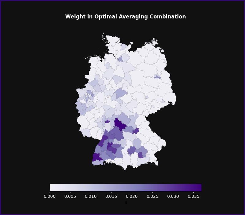
This map shows how the averaging estimator assigns weights to improve the quality of the forecast for Frankfurt. As we can see, relatively large weights are assigned to Frankfurt itself (broadly in the middle of the country), and the regions surrounding it. Hamburg (in the north), Munich (southeast), Berlin (east), and the Rhein-Ruhr region (west) also receive some weight.

Averaging Estimate

We now turn to the averaging estimates themselves. The estimated value of the target parameter (unemployment in Frankfurt) is stored in the estimate attribute:

print(averager.estimate.round(3))

-0.115

In other words, the optimally weighted forecast is that of a 0.11% decrease in the unemployment rate in the region.

We can easily compare that forecast with a forecast without any unit averaging and simply using Frankfurt-only data. IndividualUnitAverager is a convenience class that implements using target-unit only data with the same interface as other averagers:

ind_averager = IndividualUnitAverager(
    focus_function=forecast_frankfurt_jan_2020,
    ind_estimates=ind_estimates,
)
ind_averager.fit(target_id="Frankfurt")
print(ind_averager.estimate.round(3))

-0.115

In this case the individual forecast is close to the averaged one. Assuming that the individual forecast is broadly unbiased, this means that the averaged one will have lower variance due to using data on more regions.

Finally, every averager in the package (and any custom averager that inherits from BaseUnitAverager) also implements an average() method that allows one to reuse the fitted weights with a different focus function.

As a very simple example, we can define a forecaster for some other time point, say, for 12.2019:

other_target_data = (
    german_data.loc["2019-11", ["Frankfurt", "Germany_lag"]].to_numpy().squeeze()
)
other_focus_function = InlineFocusFunction(
    focus_function=lambda coef: coef[0]
    + coef[1] * other_target_data[0]
    + coef[2] * other_target_data[1],
    gradient=lambda coef: np.array([1, other_target_data[0], other_target_data[1]]),
)

We now pass the new focus function to the average() method:

averager.average(other_focus_function).round(3)

np.float64(-0.02)

Tip

It is best practice to refit weights for every focus function separately, since that allows the averager to optimally exploit the relevant similarities in the data. Reusing weights average() is only recommended with similar focus functions or when computation is expensive.