Inference I: Linear Hypotheses

Testing Linear Hypotheses. Confidence Intervals

Vladislav Morozov

Contents

• Introduction
• Background and Definitions for Testing
• One Linear Hypothesis
• General Linear Hypotheses
• Confidence Intervals and Sets
• Recap and Conclusions

Introduction

Lecture Info

Learning Outcomes

This lecture is about testing linear hypotheses and constructing asymptotic confidence intervals based on the OLS estimator

By the end, you should be able to

• Define test power, size, and test consistency
• Construct and prove properties of \(t\)- and Wald tests
• Construct valid asymptotic confidence intervals for a single coefficients

References

• 5-2, 8-2 and E4+E4a in Wooldridge (2020) (careful with the specialized formulas in 8-2, they may be a bit confusing compared to the general case in the lecture and those in E4)
• Or 7.11-7.13, 7.16, 9.1-9.9 in Hansen (2022)
• (Curious background reading): Wooldridge (2023) on the meaning of “standard error”

Reminder on the Empirical Example

Reminder: Empirical Model

Studying link between wages and (education, experience) \[ \begin{aligned}[] & [\ln(\text{wage}_i)]^{\text{(education, experience)}} \\ & = \beta_1 + \beta_2 \times \text{education} \\ & \quad + \beta_3 \times \text{experience} + \beta_4 \times \dfrac{\text{experience}^2}{100} + U_i \end{aligned} \tag{1}\]

Data: married white women from March 2009 CPS

import numpy as np
import pandas as pd
import statsmodels.api as sm

from statsmodels.regression.linear_model import OLS

# Read in the data
data_path = ("https://github.com/pegeorge/Econ521_Datasets/"
             "raw/refs/heads/main/cps09mar.csv")
cps_data = pd.read_csv(data_path)

# Generate variables
cps_data["experience"] = cps_data["age"] - cps_data["education"] - 6
cps_data["experience_sq_div"] = cps_data["experience"]**2/100
cps_data["wage"] = cps_data["earnings"]/(cps_data["week"]*cps_data["hours"] )
cps_data["log_wage"] = np.log(cps_data['wage'])

# Retain only married women white with present spouses
select_data = cps_data.loc[
    (cps_data["marital"] <= 2) & (cps_data["race"] == 1) & (cps_data["female"] == 1), :
]

# Construct X and y for regression 
exog = select_data.loc[:, ['education', 'experience', 'experience_sq_div']]
exog = sm.add_constant(exog)
endog = select_data.loc[:, "log_wage"]

Reminder: Estimation Results

results = OLS(endog, exog).fit(cov_type='HC0') # Robust covariance matrix estimator
print(results.summary())

                            OLS Regression Results                            
==============================================================================
Dep. Variable:               log_wage   R-squared:                       0.226
Model:                            OLS   Adj. R-squared:                  0.226
Method:                 Least Squares   F-statistic:                     862.5
Date:                Mon, 19 May 2025   Prob (F-statistic):               0.00
Time:                        17:37:44   Log-Likelihood:                -8152.9
No. Observations:               10402   AIC:                         1.631e+04
Df Residuals:                   10398   BIC:                         1.634e+04
Df Model:                           3                                         
Covariance Type:                  HC0                                         
=====================================================================================
                        coef    std err          z      P>|z|      [0.025      0.975]
-------------------------------------------------------------------------------------
const                 0.9799      0.040     24.675      0.000       0.902       1.058
education             0.1114      0.002     50.185      0.000       0.107       0.116
experience            0.0229      0.002     12.257      0.000       0.019       0.027
experience_sq_div    -0.0347      0.004     -8.965      0.000      -0.042      -0.027
==============================================================================
Omnibus:                     4380.404   Durbin-Watson:                   1.833
Prob(Omnibus):                  0.000   Jarque-Bera (JB):           134722.859
Skew:                          -1.401   Prob(JB):                         0.00
Kurtosis:                      20.406   Cond. No.                         219.
==============================================================================

Notes:
[1] Standard Errors are heteroscedasticity robust (HC0)

Reminder: Parameters of Interest and Estimators

Our parameters of interest:

1. \(100\beta_2\). Estimate: \(11.14\)
2. \(100\beta_3 + 20 \beta_4\). Estimate: \(1.59\)
3. \(-50\beta_3/\beta_4\). Estimate: \(36.67\)

What is the interpretation of those parameters?

Reminder: Empirical Questions

1. Does education matter at all? (up to our statistical confidence)
2. Does experience matter at all? (up to our statistical confidence)
3. Is the best amount of experience to have equal to 15 years? (up to our statistical confidence)
4. How certain are we of our estimates of target parameters?

Background and Definitions for Testing

Basic Setup: Hypotheses

Suppose that we have a model with some parameters \(\theta\) (of whatever nature)

Two competing hypotheses (statements about parameters \(\theta\)) \[ H_0: \theta\in \Theta_0 \text{ vs. } H_1: \theta \in \Theta_1 \] for some non-intersecting \(\Theta_0\) and \(\Theta_1\)

Example

• \(H_0: \beta_2=0\) (education does not affect wages)
• \(H_1: \beta_2\neq 0\) (education affects wages)

Definition of a Test

A test is a decision rule: you see the sample and then you decide in favor of \(H_0\) or \(H_1\)

Formally:

Definition 1 A test \(T\) is a function of the sample \((X_1, \dots, X_N)\) to the space \(\curl{\text{Reject } H_0, \text{Do not reject }H_0}\)

Power

Definition 2 The power function \(\text{Power}_T(\theta)\) of the test \(T\) is the probability that \(T\) rejects if \(\theta\) is the true parameter value: \[ \text{Power}_T(\theta) = P(T(X_1, \dots, X_N)=\text{Reject }H_0|\theta) \]

Test Size

Maximal power under the null has a special name

Definition 3 The size \(\alpha\) of the test \(T\) is \[ \alpha = \max_{\theta\in\Theta_0} \text{Power}_T(\theta) \]

In other words, the probability of falsely rejecting the null (type I error)

What Defines a Good Test?

The best possible test has perfect detection:

• Never rejects under \(H_0\)
• Always reject under \(H_1\)

Usually impossible in practice. Instead we ask

• Not too much false rejection under \(H_0\) (e.g. \(\leq 5\%\) of the time)
• As much rejection as possible under \(H_1\)

Test Consistency

• In finite samples, usually cannot compute \(\text{Power}_T(\theta)\)
• Instead ask that you detect \(H_1\) asymptotically

Definition 4 \(T\) is consistent if for any \(\theta\in \Theta_1\) \[ \small \lim_{N\to\infty} P(T(X_1, \dots, X_N)=\text{Reject }H_0|\theta) = 1 \]

As with estimators, we say “test” when we mean a sequence of tests, one for each sample size.

Asymptotic Size

• In finite samples, usually cannot control size exactly
• But can require it asymptotically

Definition 5 The asymptotic size \(\alpha\) of the test \(T\) is \[ \alpha = \lim_{N\to\infty} \max_{\theta\in\Theta_0} P(T(X_1, \dots, X_N)=\text{Reject }H_0|\theta) \]

One Linear Hypothesis

Example and \(t\)-Statistic

Single Example Hypothesis

Let’s start with our first empirical question:

Does education affect wages?

In the framework of Equation 1 can translate to \[ H_0: \beta_2 = 0, \quad H_1: \beta_2\neq 0 \] What are the \(\Theta_0\) and \(\Theta_1\) here if \(\theta=\bbeta\)?

How Testing Works in General

How do we construct a test/decision rule?

The basic approach to testing is surprisingly simple

1. Pick a “statistic” (=some known function of the data) that behaves “differently” under \(H_0\) and \(H_1\)
2. Is the observed value of the statistic compatible with \(H_0\)?
   • No \(\Rightarrow\) reject \(H_0\) in favor or \(H_1\)
   • Yes \(\Rightarrow\) do not reject \(H_0\)

Picking a Statistic

• In principle, can pick any statistic. Some are more “standard”
• For testing hypotheses about coefficients, there are three main classes:
  • Wald statistics: need only unrestricted estimates
  • Lagrange multiplier (LM): need restricted estimates
  • Likelihood ratio (LR): need both

Wald tests easiest to work with in linear models, but others have their uses in different contexts

Convergence of \(\hat{\beta}_2\)

Recall asymptotic distribution result for OLS estimator \[\small \sqrt{N}\left( \hat{\bbeta}- \bbeta \right) \xrightarrow{d} N(0, \avar(\hat{\bbeta})) \]

It implies (why?) that \[ \small \dfrac{\hat{\beta}_2 - \beta_2}{\sqrt{ \avar(\hat{\beta}_2)/N } } \xrightarrow{d} N\left(0, 1\right) \] where \(\avar(\hat{\beta}_2)\) is the (2, 2) element of \(\avar(\hat{\bbeta})\)

\(t\)-statistic

• Let \(\widehat{\avar}(\hat{\bbeta})\) be a consistent estimator of \(\avar(\hat{\bbeta})\)
• Let \(H_0: \beta_2 = 0\) be true

By Slutsky’s theorem (why?) it holds that \[ \small t = \dfrac{\hat{\beta}_2}{\sqrt{ \widehat{\avar}(\hat{\beta}_2)/N } } \xrightarrow{d} N\left(0, 1\right) \] \(\sqrt{ \widehat{\avar}(\hat{\beta}_2)/N }\) — standard error of \(\hat{\beta}_2\)

Decision Rule: Test

We call the following the asymptotic size \(\alpha\) \(t\)-test:

Let \(z_{1-\alpha/2} = \Phi^{-1}(1-\alpha/2)\). Then

• Reject \(H_0\) is \(\abs{t}>z_{1-\alpha/2}\)
• Do not reject \(H_0\) is \(\abs{t}\leq z_{1-\alpha/2}\)

Illustration

Illustration: Extracting Standard Errors

Can get \(\widehat{\avar}(\hat{\bbeta})\) from the results object:

(results.nobs)*results.cov_params()

	const	education	experience	experience_sq_div
const	16.406611	-0.790339	-0.411821	0.668941
education	-0.790339	0.051218	0.003703	-0.001191
experience	-0.411821	0.003703	0.036156	-0.072529
experience_sq_div	0.668941	-0.001191	-0.072529	0.156187

cov_params() extracts \(\widehat{\avar}(\hat{\bbeta})/N\)

Illustration: Doing the Test by Hand

Compute \(t\)-statistic as

t = (results.params.iloc[1])/np.sqrt(results.cov_params().iloc[1, 1])
print(t)

50.18487673168109

• Can compare t statistic to suitable quantile of the normal
• Set \(\alpha=0.05\) if want to reject at most 5% under \(H_0\) in the limit

from scipy.stats import norm
np.abs(t) > norm.ppf(1-0.05/2)

np.True_

Reject \(H_0\) in favor \(H_1: \beta_2\neq 0\) at 5% asymptotic level

Illustration: Using t_test()

Can also use

results.t_test(np.array([0, 1, 0, 0]), use_t=False)

<class 'statsmodels.stats.contrast.ContrastResults'>
                             Test for Constraints                             
==============================================================================
                 coef    std err          z      P>|z|      [0.025      0.975]
------------------------------------------------------------------------------
c0             0.1114      0.002     50.185      0.000       0.107       0.116
==============================================================================

• Reports asymptotic \(p\)-values
• Decision by comparing with the \(p\)-value
• Can reject with high confidence (very small \(p\)-value)

Illustration: \(t\) Test From the Regression Results

Regression results also print out results for \(t\)-tests of hypotheses \(H_0:\beta_k=0\)

                            OLS Regression Results                            
==============================================================================
Dep. Variable:               log_wage   R-squared:                       0.226
Model:                            OLS   Adj. R-squared:                  0.226
Method:                 Least Squares   F-statistic:                     862.5
Date:                Mon, 19 May 2025   Prob (F-statistic):               0.00
Time:                        17:37:44   Log-Likelihood:                -8152.9
No. Observations:               10402   AIC:                         1.631e+04
Df Residuals:                   10398   BIC:                         1.634e+04
Df Model:                           3                                         
Covariance Type:                  HC0                                         
=====================================================================================
                        coef    std err          z      P>|z|      [0.025      0.975]
-------------------------------------------------------------------------------------
const                 0.9799      0.040     24.675      0.000       0.902       1.058
education             0.1114      0.002     50.185      0.000       0.107       0.116
experience            0.0229      0.002     12.257      0.000       0.019       0.027
experience_sq_div    -0.0347      0.004     -8.965      0.000      -0.042      -0.027
==============================================================================
Omnibus:                     4380.404   Durbin-Watson:                   1.833
Prob(Omnibus):                  0.000   Jarque-Bera (JB):           134722.859
Skew:                          -1.401   Prob(JB):                         0.00
Kurtosis:                      20.406   Cond. No.                         219.
==============================================================================

Notes:
[1] Standard Errors are heteroscedasticity robust (HC0)

Properties

\(t\)-Test under \(H_0\): Size

What is the (asymptotic) probability of rejecting under \(H_0\)?

\[ \begin{aligned} & P\left(\text{Reject} H_0|H_0 \right) = P\left(\abs{t}>z_{1-\alpha/2} |H_0\right) \\ & = P\left( \abs{ \dfrac{\hat{\beta}_2}{\sqrt{ \widehat{\avar}(\hat{\beta}_2)/N } }}> z_{1-\alpha/2}\Bigg|H_0 \right)\\ & \to \Phi(z_{\alpha/2}) + (1- \Phi(z_{1-\alpha/2})) = \alpha \end{aligned} \]

The test has asymptotic size \(\alpha\)

\(t\)-Test under \(H_1\): Consistency

What happens to \(t\) under \(H_1\)? Suppose that \(\beta_2\neq 0\) is the true value. Can write \[ \small t = \dfrac{\hat{\beta}_2}{\sqrt{ \widehat{\avar}(\hat{\beta}_2)/N } }= \underbrace{\dfrac{\hat{\beta}_2 - \beta_2}{\sqrt{ \widehat{\avar}(\hat{\beta}_2)/N } }}_{\scriptsize \xrightarrow{d} N(0, 1)} + \underbrace{\dfrac{\beta_2}{\sqrt{ \widehat{\avar}(\hat{\beta}_2)/N } }}_{\scriptsize \xrightarrow{p} \pm \infty } \]

It follows (why?) that the \(t\)-test is consistent \[ \small P(\text{Reject } H_0|H_1) \xrightarrow{N\to\infty} 1 \]

\(t\)-Test for \(H_0:\beta_2 = c\)

More generally, can test \[ H_0: \beta_k = c \text{ vs } H_1: \beta_k \neq c \]

\(t\)-statistic \[ t = \dfrac{\hat{\beta}_k - c}{\sqrt{ \widehat{\avar}(\hat{\beta}_k)/N } } \tag{2}\]

Same decision rule: compare \(t\) to \(z_{1-\alpha/2}\)

Intuition: What the Test Does

• Under \(H_0\), the \(t\) statistic should be “well-behaved”: normal and centered at 0. Big values of \(t\)-statistic unlikely
• So if we see a big \(t\)-statistic, such a value is unlikely under \(H_0\) — evidence against \(H_0\)
• If value is large enough, we think the evidence is strong enough to be reasonably incompatible with \(H_0\) — rejection

Combined Result: \(t\)-statistics

Proposition 1 Let the assumptions for asymptotic normality of the OLS estimator hold. Let \(t\) be defined as in Equation 2. Then

1. If \(H_0: \beta_k=c\) holds, then \(t\xrightarrow{d} N(0, 1)\) The associated test has asymptotic size \(\alpha\)
2. If \(H_0: \beta_k=c\) does not hold, then \(t\xrightarrow{p}\pm\infty\). The associated test is consistent

Estimating \(\avar(\hat{\bbeta})\)

One remaining issue: how to estimate \[ \avar(\hat{\bbeta}) = \left( \E[\bX_i\bX_i']\right)^{-1} \E[U_i^2\bX_i\bX_i']\left( \E[\bX_i\bX_i']\right)^{-1} \]

Can estimate using sample analogs

1. \(\left( \E[\bX_i\bX_i']\right)^{-1}\) with \(\left( N^{-1}\sum_{i=1}^N \bX_i\bX_i'\right)^{-1}\)
2. \(\E[U_i^2\bX_i\bX_i']\) with \(N^{-1}\sum_{i=1}^N \hat{U}_i \bX_i\bX_i'\) for \(\hat{U}_i = Y_i-\bX_i'\hat{\bbeta}\)

Estimating \(\avar(\hat{\bbeta})\): Robust Standard Errors

Resulting \(\widehat{\avar}(\hat{\bbeta})\) is consistent: \[ \widehat{\avar}(\hat{\bbeta}) \xrightarrow{p} {\avar}(\hat{\bbeta}) \]

• Can use in test statistics
• \(N^{-1}\widehat{\avar}(\hat{\bbeta})\) is called robust (or heteroskedasticity robust) standard errors — specifically, HC0
• In statsmodels, we used them by called OLS(endog, exog).fit(cov_type='HC0')

General Linear Hypotheses

Example and Wald Statistic

Motivation: Need Tests for Multiple Restrictions

• \(t\)-tests allowed us to test if education mattered (\(\beta_2=0\))
• But next question is whether experience affects wages: \[ H_0: \begin{cases} \beta_3 =0\\ \beta_4 = 0 \end{cases} \quad \text{ vs } \quad H_1: \beta_3 \neq 0\text{ or } \beta_4 \neq 0 \]
• \(H_0\) has two constraints at the same time!

The “or” in \(H_1\) allows the possibility that both \(\beta_3\neq 0\) and \(\beta_4\neq 0\)

Matrix Representation of the Null

Can write our \(H_0\) as \[ \bR\bbeta = \bq \] for \[ \bR = \begin{pmatrix} 0 & 0 & 1 & 0\\ 0 & 0 & 0 & 1 \end{pmatrix}, \quad \bq =\begin{pmatrix} 0 \\ 0 \end{pmatrix} \]

Linear Hypotheses

More generally, can consider linear hypotheses of the form \[ \bR\bbeta = \bq \]

Here

• \(\bbeta\) is \(p\times 1\)
• \(\bR\) is \(k\times p\) with maximum rank — \(k\) constraints
• \(k\geq 1\) and \(k\leq p\)

Covers both example \(H_0\) we have seen so far

Towards a Statistic

Intuitive way to construct a statistic

Check the distance between \(\bR\hat{\bbeta}\) and \(\bq\)

• Reject if distance is large, do not reject if not
• How to pick “large” to ensure correct test size?
• \(\Rightarrow\) need to combine asymptotic distribution of \(\bR\hat{\bbeta}\) and distance

Asymptotic Distribution of \(\bR\hat{\bbeta}\)

Recall that \[ \sqrt{N}(\hat{\bbeta}-\bbeta)\xrightarrow{d} N(0, \avar(\bbeta)) \]

By the CMT \[ \sqrt{N}(\bR\hat{\bbeta}-\bR\bbeta) \xrightarrow{d} N(0, \bR\avar(\bbeta)\bR') \]

\(\chi^2\) Random Variables

A special useful distribution

Let \(Z_1, \dots, Z_k\) be independent \(N(0, 1)\) variables. The distribution of \(\sum_{j=1}^k Z_j^2\) is called the chi-squared distribution with \(k\) degrees of freedom (written \(\chi^2_k\))

• If \(\bZ=(Z_1, \dots, Z_k)\), then \(\bZ\sim N(0, \bI_k)\) and \(\norm{\bZ}^2 = \bZ'\bZ \sim \chi^2_k\)
• Has two ingredients we need: normality and distance

Wald Statistic

The following statistic is called a Wald statistic: \[ W = N\left( \bR\hat{\bbeta}-\bq \right)'\left(\bR\widehat{\avar}(\bbeta)\bR'\right)^{-1}\left( \bR\hat{\bbeta}-\bq \right) \tag{3}\]

• Interpretation: weighted distance
• Weighted by the inverse of the variance-covariance matrix

Decision Rule: Wald Test

We call the following the asymptotic size \(\alpha\) Wald-test:

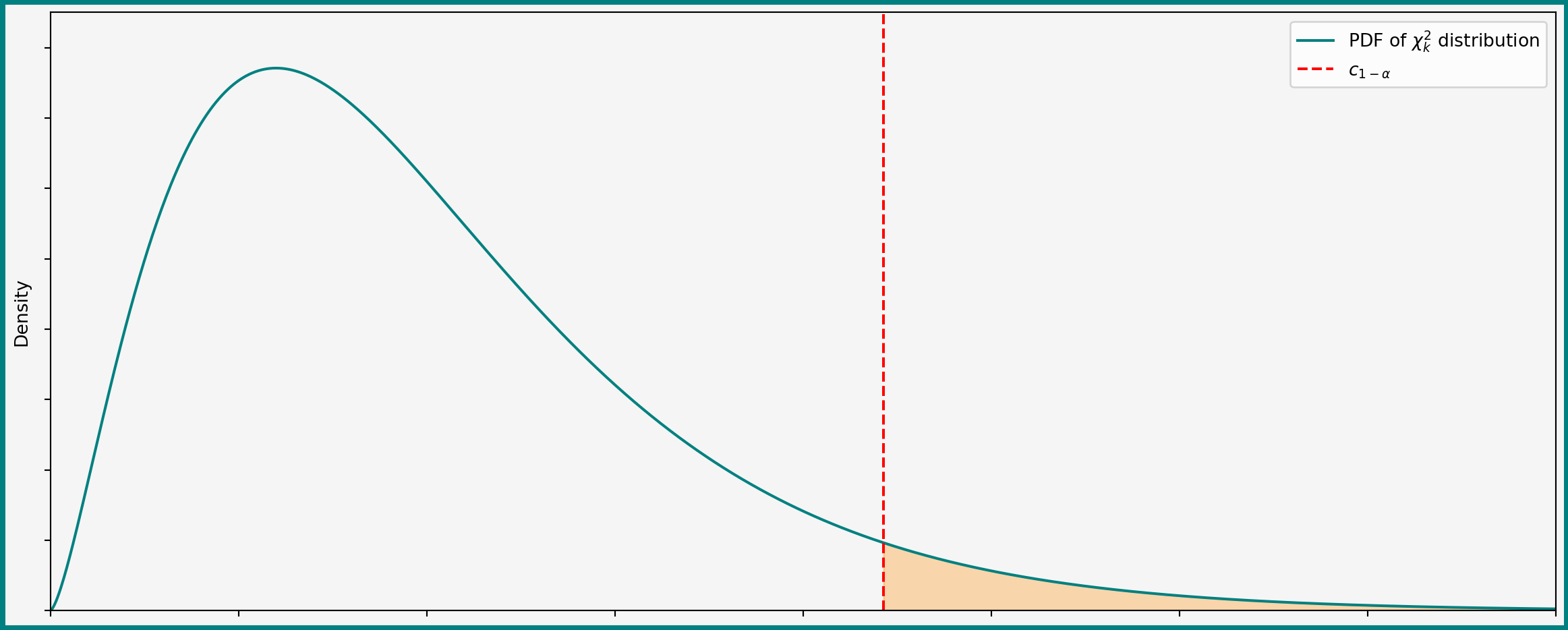
Let \(c_{1-\alpha}\) solve \(P(\chi^2_k\leq c_{1-\alpha})=1-\alpha\) where \(k\) is the number of rows and rank of \(\bR\). Then

• Reject \(H_0\) if \(W>c_{1-\alpha}\)
• Do not reject \(H_0\) if \(W\leq c_{1-\alpha}\)

Plot: PDF of \(\chi^2_k\) and Rejection Region (Shaded)

Wald and \(t\) Statistics

What if \(k=1\): only one constraint?

• Wald statistic is the square of the corresponding \(t\)-statistic (show this)
• You lose and win nothing by doing a Wald test even if you have a single hypothesis

Illustration

Effect of Experience: Expressing \(\bR\) and \(\bq\)

The results class in statsmodels has a wald_test() method

First need to define the \(\bR\) and \(\bq\) matrices:

constraint_matrix = np.array( 
    [[0, 0, 1, 0],
     [0, 0, 0, 1]]
)

rhs_vector = np.array(
    [0, 0]
)

print(constraint_matrix, '\n', rhs_vector)

[[0 0 1 0]
 [0 0 0 1]] 
 [0 0]

Effect of Experience: Using wald_test()

Then can supply \(\bR\) and \(\bq\) to wald_test() as a tuple:

wald_results = results.wald_test(
  (constraint_matrix, rhs_vector), 
  use_f=False, 
  scalar=True
)
print(wald_results)

<Wald test (chi2): statistic=270.09702395844937, p-value=2.2344799298840845e-59, df_denom=2>

• Strong evidence against \(H_0: \beta_3=\beta_4=0\)
• Experience matters for earnings

Second Example: Effect of Experience for 10 Years

Recall other parameter of interest: \(100\beta_3 + 20\beta_4\). Can ask: \[ \small H_0: 100\beta_3 + 20\beta_4 = 1.4\quad \text{ vs } \quad H_0: 100\beta_3 + 20\beta_4 \neq 1.4 \]

Can also do Wald test:

constraint_matrix = np.array( 
    [0, 0, 100, 20], 
)
rhs_vector = np.array(
    [1.4]
)
# Perform test
wald_results = results.wald_test((constraint_matrix, rhs_vector), use_f=False, scalar=True)
print(wald_results)

<Wald test (chi2): statistic=2.815200772707648, p-value=0.09337521301524496, df_denom=1>

Properties

Why Normalize by \(( \bR\avar(\bbeta)\bR')^{-1}\)

• Under \(H_0: \bR\bbeta=\bq\) it holds that \[ \sqrt{N}(\bR\hat{\bbeta}-\bq) \xrightarrow{d} N(0, \bR\avar(\bbeta)\bR') \]
• \(\norm{\bR\hat{\bbeta}-\bq}^2\) is not \(\chi^2\) unless \(\bR\avar(\bbeta)\bR'= \bI_k\)

\(\Rightarrow\) In general need to something transform \(\bR\hat{\bbeta}-\bq\) to get \(\bI_k\) asymptotic variance for \(\chi^2_k\) limit

Matrix Square Root

• Recall: if \(W\sim N(0, \sigma^2)\), then \(W/\sigma \sim N(0, 1)\)
• Similar result can be used for vectors \(\bW\sim N(0, \bSigma)\)

Just need to define “\(\sqrt{\Sigma}\)”

Proposition 2 Let \(\bSigma\) be a positive definite matrix. Then there is a unique positive definite matrix \(\bSigma^{1/2}\) such that \[ \bSigma^{1/2} \bSigma^{1/2} = \bSigma \]

Standardizing \(\bR\hat{\bbeta}\)

• So if \(\bW\sim N(0, \bSigma)\) with full rank \(\bSigma\) \[\small (\bSigma^{1/2})^{-1}\bW \sim N(0, (\bSigma^{1/2})^{-1}\bSigma(\bSigma^{1/2})^{-1}) = N(0, \bI_k) \]
• Or \[ \small ((\bSigma^{1/2})^{-1}\bW )'(\bSigma^{1/2})^{-1}\bW ) = \bW' \bSigma^{-1}\bW\sim \chi^2_k \]

We just take \(\bW=\sqrt{N}(\hat{\bbeta}-\bbeta)\) and apply the argument asymptotically and with an estimator of \(\avar(\hat{\bbeta})\)

Wald Test under \(H_0\): Size

Under the null \(H_0: \bR\bbeta=\bq\)

By Slutsky’s theorem and the above it follows \[ W = N\left( \bR\hat{\bbeta}-\bq \right)'\left(\bR\widehat{\avar}(\bbeta)\bR'\right)^{-1}\left( \bR\hat{\bbeta}-\bq \right) \xrightarrow{d} \chi^2_k \]

Hence the test is asymptotically size \(\alpha\) \[ \small P(\text{Reject } H_0|H_0) \xrightarrow{N\to\infty} \alpha \]

Wald Test under \(H_1\): Consistency

Suppose that \(H_1\) holds: \(\bR\bbeta\neq \bq\). Then

• \(\bR\hat{\bbeta}-\bq\) converges to something \(\neq 0\)
• \(\left(\bR\widehat{\avar}(\bbeta)\bR'\right)^{-1}\xrightarrow{p} \left(\bR{\avar}(\bbeta)\bR'\right)^{-1}\) by the CMT
• \(\left(\bR{\avar}(\bbeta)\bR'\right)^{-1}\) is positive definite (why?)

It follows (why?) that \(W\to+\infty\) and
\[ \small P(\text{Reject } H_0|H_1) \xrightarrow{N\to\infty} 1 \]

Combined Result: Wald Statistic and Test

Proposition 3 Let the assumptions for asymptotic normality of the OLS estimator hold. Let \(W\) be defined as in Equation 3 and let \(\bR\) have rank \(k\). Then

1. If \(H_0: \bR\bbeta=\bq\) holds, then \(W\xrightarrow{d} \chi^2_k\). The associated test has asymptotic size \(\alpha\)
2. If \(H_0: \bR\bbeta=\bq\) does not hold, then \(W\xrightarrow{p} +\infty\). The associated test is consistent

Confidence Intervals and Sets

Point vs. Interval Estimators

• Our \(\hat{\bbeta}\) is a point estimator for \(\bbeta\) — returns a single value in \(\R^p\) for each sample
• Can also consider set estimator — returns a whole set of values in \(\R^q\) as a collection of guesses for \(\bbeta\)

• Anything can be a set estimator, but we want “sensible” ones
• Leading example: confidence intervals/sets

Confidence Sets: Definition

Definition 6  

1. A \((1-\alpha)\times 100\%\) confidence set for \(\theta\) (\(\theta\in\R^p\)) is a random set \(S(X_1, \dots, X_N)\subseteq \R^p\)
   \[ \scriptsize P(\theta \in S(X_1, \dots, X_N)) = 1-\alpha \]

2. \(S(\cdot, \cdots)\) is an asymptotic \((1-\alpha)\times 100\%\) confidence set for \(\theta\) if \(\lim_{N\to\infty} P(\theta \in S(X_1, \dots, X_N)) = 1-\alpha\)

3. \(P(\theta \in S(X_1, \dots, X_N))\) is the coverage of \(S\)

Example: Confidence Intervals for \(\beta_k\)

• Can construct confidence sets based on asymptotic distribution of \(\hat{\bbeta}\)
• Example: try to construct a symmetric interval based on \(\hat{\beta}_k\) (since limit distribution is symmetric around \(\beta_k\))

Such an interval takes form \[ [\hat{\beta}_k - \hat{c}_N, \hat{\beta}_k + \hat{c}_N] \] Here \(\hat{c}_N\geq 0\) can depend on the sample and \(N\)

Picking \(\hat{c}\)

\[\scriptsize \begin{aligned} & P\left(\beta_k\in[\hat{\beta}_k - \hat{c}_N, \hat{\beta}_k + \hat{c}] \right)\\ & = P\left( - \frac{\hat{c}_N}{\sqrt{\widehat{\avar}(\hat{\beta}_k)/N} }\leq \sqrt{N} \frac{\hat{\beta}_k - \beta_k}{\widehat{\avar}(\hat{\beta}_k) }\leq \frac{\hat{c}_N}{\sqrt{\widehat{\avar}(\hat{\beta}_k)/N}} \right)\\ & \approx \Phi\left( \frac{\hat{c}_N}{\sqrt{\widehat{\avar}(\hat{\beta}_k)/N}}\right) - \Phi\left( -\dfrac{\hat{c}_N}{\sqrt{\widehat{\avar}(\hat{\beta}_k)/N}} \right) \end{aligned} \]

If we want \((1-\alpha)\times 100\%\) asymptotic coverage, pick \(\hat{c}_N = z_{1-\alpha/2} \sqrt{ \frac{\widehat{\avar}(\hat{\beta}_k)}{N} }\)

Result and Interpretation

Proposition 4 The confidence interval \[ \small \hspace{-1.6cm} S = \left[ \hat{\beta}_k - z_{1-\alpha/2} \sqrt{ \frac{\widehat{\avar}(\hat{\beta}_k)}{N} }, \hat{\beta}_k+ z_{1-\alpha/2} \sqrt{ \frac{\widehat{\avar}(\hat{\beta}_k)}{N} } \right] \tag{4}\] has asymptotic coverage \((1-\alpha)\times 100\%\)

What is the interpretation of this interval?

Connection to \(t\)-Tests: Test Inversion

There is an equivalent way to construct the confidence interval (4)

• Recall \(t\)-statistic (2) for \(H_0: \beta_k = c\)
• \(S\) is the set of all \(c\) for which the test does not reject

An example of test inversion and equivalence between testing and confidence intervals

Multivariate Confidence Sets

• Can also construct joint confidence sets for multiple parts of \(\bbeta\)
• Example approach: inverting the Wald test for \(H_0: \bbeta = \bc\)
• A bit more advanced — can read in 7.18 in Hansen (2022)

There are other ways of constructing confidence sets

Recap and Conclusions

Recap

In this lecture we

1. Reviewed key concepts from hypothesis testing
2. Discussed \(t\)- and Wald tests for linear hypotheses
3. Constructed an asymptotic confidence interval for a coefficient value

Next Questions

• What if the hypothesis is not linear in coefficients?
• How do nonlinear transformations of parameters behave?

References

Hansen, Bruce. 2022. Econometrics. Princeton_University_Press.

Wooldridge, Jeffrey M. 2020. Introductory Econometrics: A Modern Approach. Seventh edition. Boston, MA: Cengage.

———. 2023. “What Is a Standard Error? (And How Should We Compute It?).” Journal of Econometrics 237 (2): 105517. https://doi.org/10.1016/j.jeconom.2023.105517.