Learning Framework, Limits and Trade-Offs

PAC Learning, Bias-Complexity Trade-Off, and the No Free Lunch Theorem

Vladislav Morozov

Introduction

Lecture Info

Learning Outcomes

This lecture gives a framework for thinking about learning algorithms and hypothesis classes


By the end, you should be able to

  • Discuss the bias-complexity trade-off of selecting the hypothesis class
  • Define the PAC learning framework and relate PAC learning to complexity
  • Intuitively state the no free lunch theorem of learning

References


  • Chapter 1-2 in James et al. (2023)
  • Deep reading with details:
    • PAC learning: chapter 3 Shalev-Shwartz and Ben-David (2014) or chapter 2 in Mohri, Rostamizadeh, and Talwalkar (2018)
    • No-Free-Lunch theorem: chapter 5 in Shalev-Shwartz and Ben-David (2014)

This Lecture

Learning Algorithms

Think in terms of learning algorithms:

  1. Algorithm \(\Acal\) sees sample \(S=\curl{(Y_1, \bX_1), \dots, (Y_N, \bX_N)}\) and hypothesis class \(\Hcal\)
  2. Algorithm returns some \(\hat{h}_{S}^{\Acal}(\cdot)\in\Hcal\)

Example of learning algorithm: ERM

This Lecture

Want \(\Hcal\) and algorithms that “tend to” return \(\hat{h}_S(\cdot)\in \Hcal\) with “low\(R(\hat{h}_S)\)

This lecture: how to think about this matter

  • Inherent trade-off in terms of complexity of \(\Hcal\)
  • Thinking about \(\Acal\) choosing from \(\Acal\)
  • Is there a universally valid \(\Acal\)?

Bias-Complexity Tradeoff

Bayes Risk

Bayes Risk

Special name for lowest possible risk:

Definition 1 The Bayes risk is defined as \[ R^* = \inf R(h) \] across all \(h(\cdot)\) such that \(R(h)\) makes sense.

If \(h\) is such that \(R(h)=R^*\), this \(h\) is known as the Bayes predictor

Note: \(R^*\) depends on the distribution of the data

Bayes Risk Example: Independent Coin

Let \(Y=\) Heads or Tails of 50/50 coin

  • \(\bX\) — some variables that do not depend on \(Y\)
  • Risk — indicator risk


Here \(R^*=0.5\), \(\bX\) — useless for predicting

  • \(h(\bX)=Tails\) and \(h(\bX) = Heads\) both have \(R(h)=0.5\)

Bayes Risk Example: Linear Model

True model: \[ Y = \bX'\bbeta + U \] \(U\) — independent of \(\bX\) with \(\E[U]=0, \var(U) =\sigma^2\)

  • Risk: MSE
  • Best you can do — know actual \(\beta\) (next lecture and exercise)
  • \(\Rightarrow\) \(R^* = R(\bbeta) = \sigma^2\)

Excess Error


Definition 2 The excess error of a hypothesis \(h\) is defined as \[ R(h) - R^* \]

Intuition: how good we are doing with \(h\) vs. how good we can do at best

Bias-Complexity Trade-Off

Bias-Complexity Trade-Off I: Decomposition

Useful to decompose \[ \begin{aligned} R(h) - R^* = \underbrace{\left(R(h) - \inf_{h\in\Hcal} R(h) \right)}_{\text{Estimation error}} + \underbrace{\left(\inf_{h\in\Hcal} R(h)- R^* \right)}_{\text{Approximation error}} \end{aligned} \]

  • Inserted \(\inf_{h\in\Hcal} R(h)\) best you can do with \(\Hcal\)
  • Expresses key trade-off — bias-complexity trade-off

Approximation Error I

\[ \text{Approximation error} = \inf_{h\in\Hcal} R(h)- R^* \]

Shows how good \(\Hcal\) can do in terms of risk

  • Not a statistical question, studied by approximation theory
  • Increasing size/richness of hypothesis class may lower approximation error (but not raise it)

Approximation Error II

  • Example: \(\Hcal_1 \subseteq \Hcal_2\) \(\subseteq \dots\) \(\subseteq \Hcal_{\gamma} \subseteq \dots\)
  • Increasing \(\gamma\) — more complex class (e.g. allowing higher powers of polynomials)

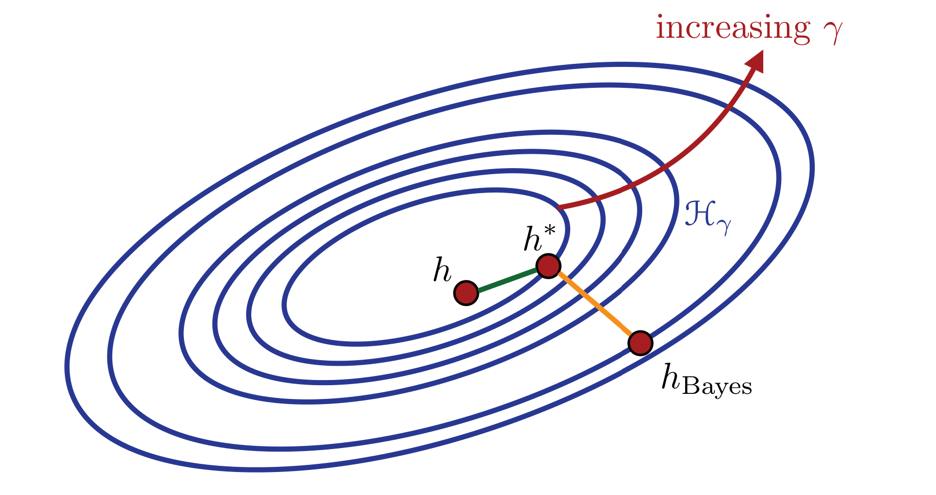
Can generally get closer to Bayes risk (e.g. by getting closer to Bayes predictor \(h_{Bayes}\))

Estimation Error I

\[ \text{Estimation error} = R(h) - \inf_{h\in\Hcal} R(h) \]

Called estimation error because usually care about \(R(\hat{h}) - \inf_{h\in\Hcal} R(h)\) where \(\hat{h}\) is selected based on data

Controlled by

  • Learning algorithm: how is \(\hat{h}\) chosen
  • Complexity of \(\Hcal\)
  • Amount of data available for learning

Estimation Error and Overfitting

How does estimation error depend on complexity of \(\Hcal\)?

  • In general: more difficult to control with larger \(\Hcal\)
  • Intuitively:
    • Sample is finite: only limited information
    • Harder to choose well with more options
  • Related to overfitting: choosing a too complex \(\hat{h}\): low risk on training sample, poor generalization

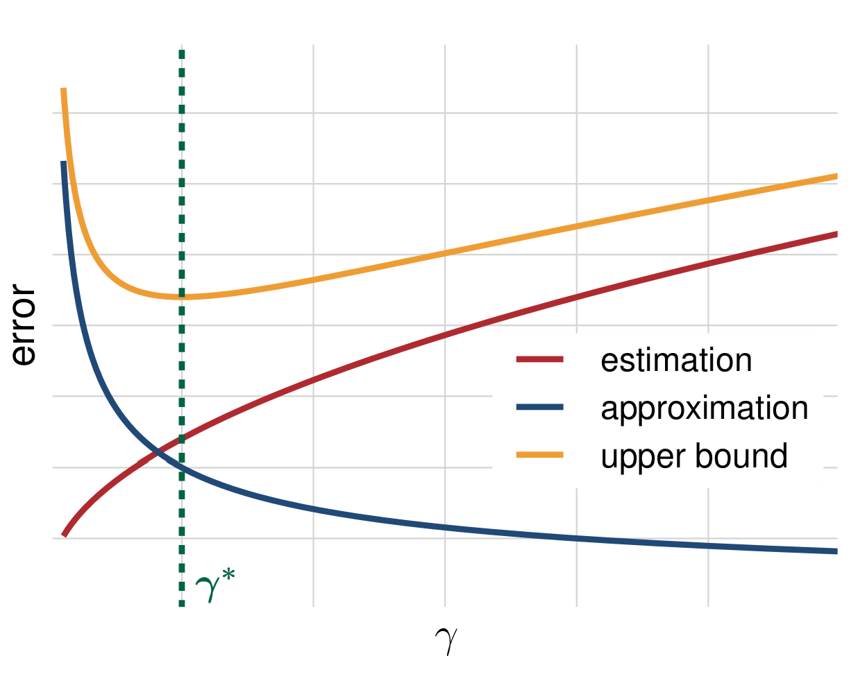
Bias-Complexity Trade-Off II: Visually

  • Increasing complexity: approximation error \(\Downarrow\), estimation error \(\Uparrow\) (more or less)
  • Creates a trade-off
  • Finding optimal point — art. Depends on the specific problem (more on that later)

Underfitting

If approximation error dominates

  • \(\Hcal\) not complex enough
  • Called underfitting


Solution: use a richer \(\Hcal\)

Overfitting

Estimation error dominates if \(\hat{h}\) chosen poorly

  • Usual source: overfitting
  • Also maybe due to optimization issues

Solutions:

  • Use a less complex \(\Hcal\)
  • Add penalty to empirical risk/objective to punish more complex models (e.g. \(L^1\) or \(L^2\) penalties from last time)

PAC Learning

Motivation

Mentioned before: approximation error studied by approximation theory, not a statistical question


How is estimation error studied?

  • Part of “core” statistical learning theory
  • Basic framework for thinking — probably approximately correct (PAC) learning
  • Introduce it now and talk more about generalization

Reminder: Notation

Pieces of learning:

  • Algorithm \(\Acal\)
  • Sample \(S=\curl{(Y_1, \bX_1), \dots, (Y_N, \bX_N)}\)
  • Hypothesis class \(\Hcal\)


\(\Acal\) selects some \(\hat{h}_S^{\Acal}\) from \(\Hcal\) after seeing \(S\)

Randomness in Generalization and Estimation Errors

Generalization error (risk) of \(\hat{h}^{\Acal}_S\): \[ R(\hat{h}^{\Acal}_S) = \E_{(Y, \bX)}\left[ l(Y, \hat{h}_S(\bX)) \right] \]

  • Expectation over new independent point \((Y, \bX)\), not over the sample (\(\hat{h}^{\Acal}_S\) fixed for the expectation)!
  • \(\Rightarrow R(\hat{h}^{\Acal}_S)\) is random because it depends on sample \(S\)
  • \(\Rightarrow\) estimation error \(R(\hat{h}^{\Acal}_S) - \inf_{h\in\Hcal}R(h)\) also random

PAC: Intuitive Form

  • Want to have \(R(\hat{h}^{\Acal}_S) - \inf_{h\in\Hcal}R(h)\) small — less than some \(\varepsilon\) (to be approximately correct)
  • Want this to happen for most samples, at least share \(1-\delta\) of possible samples of size \(m\) (for it to happen probably)
  • Want it to hold regardless of the distribution of data


PAC learning (Valiant 1984) combines these requirements

PAC: Simplified Definition

Definition 3 \(\Acal\) is a PAC learning algorithm if for any \(\varepsilon>0, \delta>0\) there exists a sample size \(m\) such that for all distributions of data \(\Dcal\) and all samples of size \(m\) from \(\Dcal\) it holds that \[ P_{S}\left(R(\hat{h}^{\Acal}_S) - \min_{h\in\Hcal} R(h) \leq \varepsilon \right) \geq 1-\delta, \] where \(\hat{h}_S\) is the hypothesis selected by \(\Acal\) from \(\Hcal\)

PAC: Discussion

  • PAC learning algorithms are good because they control estimation error
  • Complexity and PAC:
    • If \(\Hcal\) is more complex, then \(m\) is larger — need larger samples to achieve same \(\varepsilon\) and \(1-\delta\)
    • Formal justification for why more complex \(\Hcal\) are harder to learn
  • “Bad” PAC results do not mean bad performance in practice (e.g. deep neural networks)

No Free Lunch Theorem

Motivation

So far: talking on the level of a single algorithm \(\Acal\)

  • Trade-offs you face in terms of bias vs. complexity
  • How to express the ability to control estimation error (PAC)


Do we even need to study and use different algorithms?

Given a risk function \(R\), is there a universal learning algorithm?

No Free Lunch: Intuitive Form

No free lunch theorems: no such algorithm exists

NFL theorems (Wolpert 1996) look like this:

  • Fix risk \(R(\cdot)\) and any algorithm \(\Acal\) that returns \(\hat{h}_S^{\Acal}\) after seeing a sample \(S\)
  • There exist a data distribution such that
    • \(R(\hat{h}_S^{\Acal})\) is “big”
    • There exists another \(h\) such that \(R(h)=0\)

No Free Lunch: Simple Example

Proposition 1 Let \(\Acal\) be any learning algorithm for binary classification under indicator loss with \(X\in \R\). Let \(m\) be any sample size. There exists some distribution \(\Dcal\) of data such that

  • There exists a hypothesis \(h\) such that \(R(h^*)=0\)
  • With probability of at least \(1/7\) over samples \(S\) of size \(m\) \[ \small R(\hat{h}^{\Acal}_S) \geq 1/8. \]

No Free Lunch: Discussion

  • What NFL theorems show: every algorithm fails somewhere
  • What NFL theorems do not show:
    • NFL is not about some problems being harder (with worse risk)
    • Specifically constructs a failure of \(\Acal\) where another algorithm succeeds

No Free Lunch: Implications

You always need some prior (domain) knowledge for successful learning

Prior knowledge expressed in terms of selecting \(\Hcal\), \(\Acal\), imposing penalties, choosing predictors, network architecture, etc.

  • Also: NFL — no universal automatic way to select \(\Hcal\)
  • \(\Rightarrow\) no automatic way of finding the optimal bias-complexity trade-off

Recap and Conclusions

Recap


In this lecture we

  1. Discussed the bias-complexity trade-off
  2. Introduced PAC-learning
  3. Discussed limitations of learning in form of the no free lunch theorems

Next Questions


With the theoretical foundations of the last three sections, can now deep dive into both theoretical and practical aspects:

  • How does a practical learning problem look like?
  • How do you estimate the risk of the chosen hypothesis?
  • Which algorithms are appropriate in which case?
  • How to select \(\Hcal\)?

Etc.

References

James, Gareth, Daniela Witten, Trevor Hastie, Robert Tibshirani, and Jonathan E. Taylor. 2023. An Introduction to Statistical Learning: With Applications in Python. Springer Texts in Statistics. Cham: Springer.
Mohri, Mehryar, Afshin Rostamizadeh, and Ameet Talwalkar. 2018. Foundations of Machine Learning. The MIT Press. https://doi.org/10.5555/3360093.
Shalev-Shwartz, Shai, and Shai Ben-David. 2014. Understanding Machine Learning. 1st ed. West Nyack: Cambridge University Press.
Valiant, Leslie G. 1984. “A Theory of the Learnable.” Communications of the ACM 27 (11): 1134–42. https://doi.org/10.1145/1968.1972.
Wolpert, David H. 1996. “The Lack of A Priori Distinctions Between Learning Algorithms.” Neural Computation 8 (7): 1341–90. https://doi.org/10.1162/neco.1996.8.7.1341.