Components of an ML Problem
Risk and Hypothesis Classes
Introduction
Lecture Info
Learning Outcomes
This lecture is about the key components of a prediction problem
By the end, you should be able to
- Define loss and risk functions
- View optimal prediction as a problem of generalization
- Discuss practical issues arising during risk minimization (overfitting, computational challenges, etc)
References
Setting
Setting
Will work only in supervised setting in this course
Setup:
- Sample of \(N\) examples
- All samples labeled with label \(Y_i\)
- Features — vector of \(p\) explanatory variables \(\bX_i\)
Notice the vocabulary: ML vocabulary established and sometimes different from causal inference vocabulary
Regression and Classification
Two main kinds of supervised problems:
- Regression: \(Y\) continuous or close to it
- Classification: finite set of values for \(Y\)
- Values of \(Y\) not necessarily ordered
- E.g. binary classification: \(Y\) can have two values (e.g. 0 and 1)
- Multiclass classification: \(Y\) can have more than two values (e.g. “bus”, “train”, “plane”)
Loss and Risk
Key Goal of Prediction
Key goal of prediction — predicting \(Y\) “well”
- Other aspects: scalability, computational efficiency, interpretability
- Difference from causal inference: there interested in causal effect of some \(X_{ij}\) on \(Y_i\)
- Most important: correct identification
- Only then efficiency/fit
How to define “well”?
Loss and Risk
Quality of prediction measured with risk function
Let \(h(\bX)\) be a prediction of \(Y\) given \(\bX\) (hypothesis)Definition 1 Let the loss function \(l(y, \hat{y})\) satisfy \(l(y, \hat{y})\geq 0\) and \(l(y, y)=0\) for all \(y, \hat{y}\).
The risk function of the hypothesis (prediction) \(h(\cdot)\) is the expected loss: \[ R(h) = \E_{(Y, \bX)}\left[ l(Y, h(\bX)) \right] \]
Examples of Risk Functions
- Indicator risk: \(\E[\I\curl{Y\neq h(\bX)}]\)
- Most common in classification
- Same price for any kind of error
- Mean squared error \(\E[(Y - h(\bX))^2]\) and mean absolute error \(\E[\abs{Y- h(\bX)}]\)
- Asymmetric risks such as linex: \(\E[\exp(\alpha[Y-h(\bX)]) - \alpha[Y-h(\bX)]-1]\) for \(\alpha\in \R\)
- If \(\alpha>0\), punishes overprediction more than underprediction
Interpretation: Generalization Error
Risk measures how well the hypothesis \(h\) performs on unseen data — generalization error
Example: indicator risk: \[ \E[\I\curl{Y\neq h(\bX)}] = P(Y\neq h(\bX)) \] Probability of incorrectly predicting \(Y\) with \(h(\bX)\) — where \(Y\) and \(\bX\) are a new observation
Choosing a Risk Function
Risk function
- Key metric of interest
- Reflects what is directly important in your context:
- Impact of new policy on revenue
- Diagnosing cancer correctly
- Flagging fraud
- \(\Rightarrow\) choice of risk function — not a statistical question, but question of context
Risk is not necessarily the criterion function used for estimation
Empirical Risk and Hypotheses
Challenges in Choosing \(h(\cdot)\)
Ideally want to choose best possible \(h(\cdot)\): \[ \small h(\cdot) \in \argmin_{h} R(h(\cdot)) \tag{1}\] But challenges:
- Don’t know \(R(\cdot)\) — it depends on the true population distribution of data
- Can’t practically minimize over the class of all functions
Empirical Risk
Empirical Risk
Sample version of risk — empirical risk : \[ \small \hat{R}_N(h) = \dfrac{1}{N}\sum_{i=1}^N l(Y_i, h(\bX_i)). \] Average over sample \(S = \curl{(Y_1, \bX_1), \dots, (Y_N, \bX_N)}\)
Empirical Risk Minimization
Minimizing \(\hat{R}_N\) — empirical risk minimization (ERM): \[ \small \hat{h}^{ERM}_S \in \argmin_{h} \hat{R}_N(h) \]
- ERM — theoretically among the most central learning algorithms
- Closely tied to the actual problem of interest
- Sometimes computationally infeasible (more on that later)
Hypothesis Classes
Issue with Minimizing Over All Functions
Minimization in Equation 1 — over all \(h\) such that the risk makes sense
Issues:
- Computation: usually cannot search through such a large class
- Theoretical: can overfit: fit the sample too well, generalize to unseen data poorly (more on that later)
Hypothesis Classes
Solution: look for \(h\) in some hypothesis class \(\Hcal\)
Then ERM: \[ \hat{h}_N^{ERM} \in \argmin_{h\in\Hcal} \hat{R}_N(h) \]
Careful with terminology
“Hypothesis” in ML — basically a model with specific coefficients.
Do not confuse with hypotheses in inference
Examples of Hypothesis Classes I
Popular class: linear predictors/classifiers
Regression: \[ \small \Hcal= \curl{h(\bx)=\varphi(\bx)'\bbeta: \bbeta\in \R^{\dim(\varphi(\bx))} } \]
Binary classification: \[ \small \Hcal = \curl{h(\bx) = \I\curl{\varphi(\bx)'\bbeta \geq 0}: \bbeta\in \R^{\dim(\varphi(\bx))} } \]
\(\varphi(\bx)\) — some known transformation of predictors
Example of ERM: Linear Regression I
Already know an example of ERM with specific hypothesis class — linear regression
Problem elements:
- Risk — mean squared error
- Hypothesis class \(\Hcal\): linear combinations of \(\bX\) of form \(h(\bx)=\bx'\bbeta\)
- Assume \(\bX'\bX\) invertible
Example of ERM: Linear Regression II
Empirical risk minimizer: \[ \begin{aligned} \hat{h}(\bx) & = \bx'\hat{\bbeta}, \\ \hat{\bbeta} & = \argmin_{\bb} \dfrac{1}{N}\sum_{i=1}^N (Y_i - \bX_i'\bb)^2 = (\bX'\bX)^{-1}\bX'\bY \end{aligned} \]
- Optimizing over \(\Hcal\) — same as optimizing over \(\bb\)
- OLS — example of ERM procedure
Inductive Bias
Choice of \(\Hcal\) — part of choice of inductive bias
Definition 2 Inductive bias is the set of assumptions that the learning algorithm uses to generalize to unseen data
Examples:
- Family of functions linking \(\bX\) and \(Y\) (e.g. linear in \(\varphi(\bX)\))
- Or: value of \(Y\) nearly constant in small neighborhoods (as used by \(k\)-nearest neighbors regressors and classifiers)
Examples of Hypothesis Classes II: Trees I
Another approach taken by decision trees
Trees:
- Divide predictor space into regions
- Predict the same value for all values in a region
- Divisions computed using recursive binary splitting
Can use both for regression and classification
Examples of Hypothesis Classes II: Trees II
- Split the predictor space one variable at a time
- Return same value on each rectangle \(R_k\)
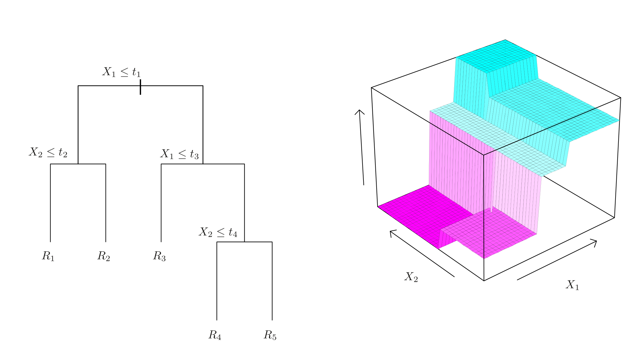
Illustration: figure 8.3 in James et al. (2023)
Beyond Simple ERM
Challenges with ERM
ERM over \(\Hcal\) \[ \small \hat{h}^{ERM}_S \in \argmin_{h \in \Hcal} \hat{R}_N(h) \]
Can still have some challenges:
- We may want to make minimization prefer some \(h\) over others in \(\Hcal\)
- ERM may be computationally infeasible
Penalties
Why Prefer Simpler Models?
- Philosophically: Occam’s razor
- Practically: overfitting
- A more complex hypothesis can fit training data better
- But may fit the data too closely — algorithm starts to learn noise together with data
- Learning noise — unhelpful for generalization
Story with overfitting is more complicated thanks to “double descent”, seen especially in deep learning
Overfitting: Visual Example
Visual example — binary classification (red, blue) with two features
- Outlined dots — unseen
- Green — complex hypothesis, perfect on training sample
- Black line — less complex
- Green line generalizes worse than black (more errors on unseen points)

Image from Wikipedia
Motivational Example
Suppose: \(X\) scalar, \(\Hcal\) — polynomials up to 10th degree \[ \small \Hcal= \curl{h(x) = \sum_{k=0}^{10} \beta_k x^k, \beta\in \R^{11} } \]
- Higher degree — more complicated explanation
- Occam’s razor — prefer simpler explanation
How to prefer simpler explanations with ERM?
Penalties: Regularization
General answer
- Create some positive measure of complexity \(\Pcal(h)\)
- Add to empirical risk as a regularization (penalty) term
\[ \small \hat{h}\in\argmin_{h\in\Hcal} \hat{R}_N(h) + \lambda \Pcal(h) \tag{2}\]
\(\lambda\geq 0\) — fixed penalty parameter, controls balance between penalty and risk
Example: Ridge and Lasso
Hypothesis set: \(\Hcal= \curl{h(\bx)= \varphi(\bx)'\bbeta: \bbeta\in \R^{\dim(\varphi(\bx))}}\)
Popular penalties:
- Ridge (\(L^2\)): \(\norm{\bbeta}_2^2 = \sum_{k} \beta_k^2\)
- Lasso (\(L^1\)): \(\norm{\bbeta}_1 = \sum_{k} \abs{\beta}_k\)
- Elastic net: \(\norm{\beta}_1 + \kappa \norm{\beta}_2^2\). Here \(\kappa\) — relative strength of \(L^1\) and \(L^2\)
Arise often and used in many models (see lecture on predictive regression)
Penalty Size: \(\lambda\)
\(\lambda\) in Equation 2:
- Is a hyperparameter — parameter not chosen during training (choosing \(h\))
- Can interpret as Lagrange multiplier for constraint \(\Pcal(h) = c\) for some \(c\)
- Chosen during the validation step using separate data or cross-validation
Surrogate Losses
Surrogate Losses
- ERM good: connected to minimizing actual risk
- But sometimes ERM computationally infeasible
- Solution: minimize some easier “surrogate” objective to find \(\hat{h}(\cdot)\)
Important
Quality of \(\hat{h}(\cdot)\) evaluated in terms of actual risk regardless
Example: Logit I
Example: binary classification (\(Y=0, 1\)) with a logit classifier based on some \(\bX\)
Classifiers indexed by \(\bbeta\): \[ \begin{aligned} h(\bx) & = \I\curl{ \Lambda( \bx'\bbeta ) \geq 0.5 }, \\ \Lambda(x) & = \dfrac{1}{1+\exp(-x)} \end{aligned} \] \(\Lambda\) — CDF of the logistic distribution
Example: Logit II
ERM to learn best \(\bbeta\) (with indicator/misclassification risk) \[ \hat{\bbeta}^{ERM} \in \argmin_{\bbeta} \dfrac{1}{N} \sum_{i=1}^N \I\curl{ Y_i\neq \I\curl{ \Lambda( \bX_i'\bbeta ) \geq 0.5 } } \]
Hard minimization — function is not even continuous in \(\bbeta\)
Example: Logit III
Instead of ERM can maximize the (quasi) log likelihood: \[ \small \hat{\bbeta}^{QML} = \argmax_{\bbeta} \sum_{i=1}^N\left[Y_i \log(\Lambda( \bX_i'\bbeta )) + (1-Y_i) \log\left( 1 - \Lambda( \bX_i'\bbeta ) \right) \right] \]
Original justification — a very specific data generating process (see 17.1 in Wooldridge (2020)).
In prediction, using maximum likelihood does not mean that you believe it — quasi means likelihood doesn’t necessarily reflect true process
Hypothesis quality checked using the actual risk — probability of predicting \(Y\) incorrectly
Example: Logit IV
- Maximizing likelihood much easier
- Can write \(\hat{\bbeta}^{QML}\) as \[ \small \begin{aligned} \hat{\bbeta}^{QML} & = \argmin_{\bbeta} \dfrac{1}{N}\sum_{i=1}^N l(Y_i, \bbeta), \\ l(Y_i, \bb) & = - \left[Y_i \log(\Lambda( \bX_i'\bbeta )) + (1-Y_i) \log\left( 1 - \Lambda( \bX_i'\bbeta ) \right) \right] \end{aligned} \] \(\hat{\bbeta}^{QML}\) — ERM under negative likelihood loss
- Likelihood loss — “surrogate” for the target (indicator)
Example: Logit V
- Recall: likelihood “\(\approx\)” probability of sample given \(\bbeta\)
- \(\Rightarrow\) Another interpretation — logit classifier is learning to predict class probabilities (classes — 0, 1): \[ \widehat{P}(Y=1|\bX=x) = \Lambda(\bx'\hat{\bbeta}^{QML}) \]
- We then compare predicted probabilities to the decision threshold 0.5
Some algorithms can return such scores or probabilities (e.g. SVMs, logit-like). Some algorithms can only return the final labels (e.g. classification trees)
Recap and Conclusions
Recap
In this lecture we
- Defined loss and risk
- Framed optimal prediction as risk minimization
- Introduced empirical risk minimization + penalties and surrogate losses
Next Questions
- How do you estimate the risk of the chosen hypothesis?
- Is there a universally valid way to predict?
- What properties do we want our learning algorithms to have?
References
Risk and Hypothesis Classes