Different people react differently to same change in \(\bx\)
Average effect of going from \(\bx_1\) to \(\bx_2\) is \((\bx_2-\bx_1)'\E[\bbeta_i]\)
Want to learn \(\E[\bbeta_i]\)
Issue with FE Estimators and This Lecture
Last time proved that under model (1) FE estimators estimate weighted average \[
\hat{\bbeta}^{FE} \xrightarrow{p} \E[\bW(\tilde{\bX}_i)\bbeta_i]
\] Outside of RCTs usually \(\E[\bW(\tilde{\bX}_i)\bbeta_i]\neq \E[\bbeta_i]\)
Weights \(\bW(\cdot)\) “nice”: positive definite and integrate to 1
But \(\bW(\cdot)\) — difficult to interpret
This lecture — way to estimate \(\E[\bbeta_i]\) with panel data
Empirical Motivation
Last time discussed relationship between pollution and labor market outcomes using US county-level data
What if pollution effect differs between counties?
E.g. due to different population characteristics (age, health, …)
Would be an example of model (1). FE estimate from last time would be \(\E[\bW(\tilde{\bX})\bbeta_i]\)
What is \(\E[\bbeta_i]\)?
Theory
Construction
Model and Data
Vector form of realized outcomes in model (1): \[
\bY_i = \bX_i\bbeta_i + \bU_i
\]\(\bbeta_i\) — \(p\)-vector. Interested in \(\E[\bbeta_i]\)
Assumption: \(T\geq p\)
At least as many observations as there are coefficients
Last time assumed that two random intercepts sufficient to capture important unobserved components:
County-season
State-year
Unit of analysis effectively county in given season (e.g. King County in summer is a single \(i\))
After that assumed that effect of pollution was same between places
Allowing Different Effects
What if pollution effects differ between counties and seasons?
Specify model as example of (1) \[ \small
Y_{it}^{\bx} = \alpha_i + \beta_i\text{Smoke Days}_{it} + \text{State-Year FE} + U_{it}
\]\(i\) — county in given season; \(t\) — years
Keep state-year effect to capture “global” effects
\(\E[\beta_i]\) — object of interest
Estimation and Results
Estimation Steps
Our approach to estimating with \(\E[\beta_i]\) with mean group estimator:
Eliminate state-year FE
Compute all individual effects
Compute MG estimator
Step (1) not part of MG estimation, included here due to our model
Eliminating State-Year FE
How do we eliminate state-year random intercept?
One-way within transformation:
Average inside each (state-year)
Take out that average from \(Y_{it}\) and \(X_{it}\)
Loading, preparing data. Eliminating state-year random intercepts
Mean group not implemented anywhere (to the best of my knowledge), but very easy to do by hand
With a for-loop
By grouping the data based on county-quarter ID
A small function for running individual regressions:
Function for running unit-level OLS
def run_individual_regression(county_quarter_df: pd.DataFrame) -> np.float64:""" Compute the OLS coefficient for 'smoke_days_no_state_year' on 'diff_payroll' for a given county-quarter DataFrame. Parameters ---------- county_quarter_df : pd.DataFrame DataFrame containing at least the columns 'diff_payroll' and 'smoke_days_no_state_year'. Returns ------- np.float64 Estimated coefficient for 'smoke_days_no_state_year'. Raises ------ KeyError If required columns are missing. ValueError If regression cannot be performed (e.g., insufficient data). """try: y = county_quarter_df['diff_payroll_no_state_year'] X = sm.add_constant(county_quarter_df['smoke_days_no_state_year']) model = sm.OLS(y, X) results = model.fit() coef = results.params['smoke_days_no_state_year']return coefexceptKeyErroras e: # Column missingraiseValueError(f"Required column missing: {e}")exceptValueErroras e: # Regression-related issuesraiseValueError(f"Regression could not be performed: {e}")
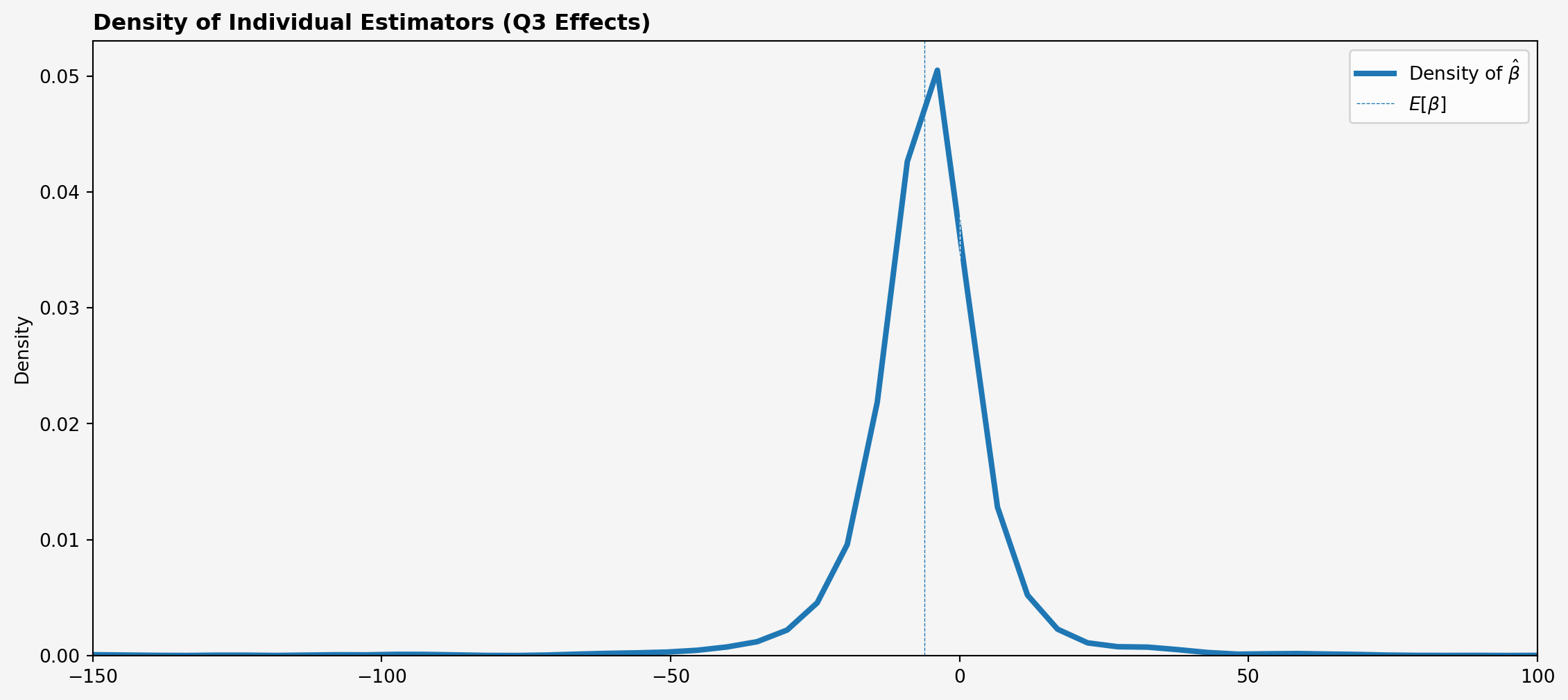
Large standard deviation! Cannot reject \(\E[\beta_i]=0\) — do not have the finding of Borgschulte, Molitor, and Zou (2024) in this model
Visualizing Density of \(\hat{\beta}_i\)
Why Such a Large Standard Deviation?
Density of \(\hat{\beta}_i\) wide, could be due to two reasons:
Large \(\var(\beta_i)\). Means \(\E[\beta_i]\) would be difficult to estimate even without estimation noise
Large \(\var((\bX_i'\bX_i)^{-1}\bX_i'\bU_i)\) — estimation noise dominates
In first case collecting more \(T\) would not help
Visualizing Geography of Effects
Recap and Conclusions
Recap
In this lecture we
Proposed the mean group estimator as an approach to estimating \(\E[\bbeta_i]\)
Discussed its asymptotic properties
Next Questions
What if we don’t care about causal parameters and only want to predict outcomes?
When does strict exogeneity fail? What is the impact of that failure?
How to work with panel data in nonlinear settings?
References
Borgschulte, Mark, David Molitor, and Eric Yongchen Zou. 2024. “Air Pollution and the Labor Market: Evidence from Wildfire Smoke.”Review of Economics and Statistics 106 (6): 1558–75. https://doi.org/10.1162/rest_a_01243.
Morozov, Vladislav. 2025. “Econometrics with Unobserved Heterogeneity.”Econometrics with Unobserved Heterogeneity. https://zenodo.org/doi/10.5281/zenodo.15459848. https://doi.org/10.5281/ZENODO.15459848.