The Hidden Delta Method in statsmodels (A Worked Example)
Using the delta method in Python with statsmodels for nonlinear inference: a practical example of confidence intervals and tests
This post demonstrates how to use the delta method in statsmodels for inference on nonlinear functions of parameters. Surprisingly, this functionality is not documented. I provide a practical example with a wage regression, showing how to create a suitable delta method instance and use it for computing confidence intervals and tests.
- Empirical Example: When do Earnings Peak?
- The Delta Method: Core Result and Why It Matters
- A Worked Example
The delta method is a core tool in applied causal inference. It’s what allows you to construct confidence intervals and tests for nonlinear functions of model parameters, like elasticities, marginal effects, or maxima.
If you want to use in Python, though, you may quickly run into a wall. A search for “delta method Python” doesn’t turn up much. That’s surprising, since it turns out it is fully implemented in statsmodels, one of the most important stats packages. When I wanted to use it myself, I found the functionality undocumented and effectively unknown. I only discovered it by digging through the source code.
This post walks through a worked example using that hidden functionality. It focuses on how to apply the delta method in practice with statsmodels: estimating nonlinear transformations, computing standard errors, building confidence intervals, and running Wald tests in a real setting.
This is not a critique of statsmodels, which is a fantastic and foundational open-source project. I think of this post as an informal, example-driven starting point for broader documentation. Anyone (myself included) could consider contributing directly.
The full Python code in this post can be found in the blog GitHub repo.

Empirical Example: When do Earnings Peak?
How much work experience maximizes yearly earnings? That’s the question we’ll use as our running example.
To answer it, we model log wages as a function of education and experience using the following potential outcomes framework: \[\begin{aligned}[] & [\ln(\text{wage}_i)]^{\text{(education, experience)}} \\ & = \theta_1 + \theta_2 \times \text{education} \\ & \quad + \theta_3 \times \text{experience} + \theta_4 \times \dfrac{\text{experience}^2}{100} + U_i. \end{aligned}\]
Here, \(\theta_j\) are unknown parameters and \(U_i\) is some “nice” unobserved term. We divide experience\({}^2\) by 100 to ensure numerical stability.
The squared term captures the empirical fact that earnings typically rise with experience, then decline later in a career. As a consequence, we expect there to be an amount of experience at which the earnings peak. The experience level that maximizes expected log wage is: \[f(\theta) = -50\frac{\theta_3}{\theta_4}.\]
This \(f(\theta)\) is our key parameter of interest. We can estimate it with \(f(\hat{\theta})\) where \(\hat{\theta}\) is the OLS or any other estimator of the \(\theta\)s.
How do we measure uncertainty given that \(f(\theta)\) is a nonlinear transformation of the vector of \(\theta\)s? The delta method gives us exactly what we need: a way to quantify uncertainty and conduct inference on \(f(\theta)\).
The Delta Method: Core Result and Why It Matters
First, a quick overview of the essential result. If you’re looking for more details, checking out some references (here are some undergraduate slides from my teaching) can be helpful, but I’ll cover the key statement here.
Statement of the Delta Method
In short, the delta method lets us derive the asymptotic distribution of a function of an estimator — based on the estimator’s own asymptotic distribution. Suppose we know the asymptotic distribution of an estimator \(\hat{\theta}\). We’re interested in a smooth transformation \(f(\hat{\theta})\), such as the level of experience that maximizes expected earnings. The delta method tells us how \(f(\hat{\theta})\) behaves in large samples.
The most common version is the first-order delta method. Suppose \(\hat{\theta}\) is a consistent and asymptotically normal estimator: \[\sqrt{n}(\hat{\theta}-\theta)\xrightarrow{d} N(0, \Sigma),\]
where \(n\) is the sample size and \(\Sigma\) is the asymptotic variance matrix of \(\hat{\theta}\).
Let \(f: \mathbb{R}^{\mathrm{dim}(\theta)} \to \mathbb{R}\) be a differentiable function with nonzero gradient at \(\theta\), i.e., \(\nabla f(\theta) \ne 0\). Then: \[\sqrt{n}(f(\hat{\theta})- f(\theta)) \xrightarrow{d} N(0, \nabla f(\theta)' \Sigma \nabla f(\theta)).\]
In other words, we’ve extended the convergence result from \(\hat{\theta}\) to the transformed quantity \(f(\hat{\theta})\).
More advanced versions of the delta method allow more general functions \(f\), estimators \(\hat{\theta}\) in abstract parameter spaces, and convergence to non-normal limits. For our empirical examples (and the version in statsmodels), the above formulation will suffice.
Why the Delta Method Matters
Why is the delta method useful? Asymptotic inference relies on convergence results like: \[\sqrt{n}(f(\hat{\theta})-f(\theta))\xrightarrow{d} N(0, \mathrm{avar}(\hat{\theta})).\]
Once this form is established, standard tools apply immediately. We can construct confidence intervals and tests regarding \(f(\theta)\) in the same manner as when dealing with \(\theta\).
What the delta method does is give us the machinery to reach the desired convergence result. It also describes the asymptotic variance of \(f(\hat{\theta})\).
A Worked Example
The Data and the Estimate
Recall our empirical question: how many years of experience maximize yearly earnings?
To estimate the relationship between wages, experience, and education, we use data from the 2009 Current Population Survey (CPS), focusing on married white women with present spouses to create a relatively homogeneous sample.
For brevity, I’ll hide the data preparation section, but feel free to click below to see the details: Click to see data preparation import numpy as np
import pandas as pd
import statsmodels.api as sm
from statsmodels.regression.linear_model import OLS
# Read in the data
data_path = ("https://github.com/pegeorge/Econ521_Datasets/"
"raw/refs/heads/main/cps09mar.csv")
cps_data = pd.read_csv(data_path)
# Generate variables
cps_data["experience"] = cps_data["age"] - cps_data["education"] - 6
cps_data["experience_sq_div"] = cps_data["experience"]**2/100
cps_data["wage"] = cps_data["earnings"]/(cps_data["week"]*cps_data["hours"] )
cps_data["log_wage"] = np.log(cps_data['wage'])
# Retain only married women white with present spouses
select_data = cps_data.loc[
(cps_data["marital"] <= 2) & (cps_data["race"] == 1) & (cps_data["female"] == 1), :
]
# Construct X and y for regression
exog = select_data.loc[:, ['education', 'experience', 'experience_sq_div']]
exog = sm.add_constant(exog)
endog = select_data.loc[:, "log_wage"]
With our data prepared, we estimate the wage regression using OLS and produce a standard statsmodels results table:
results = OLS(endog, exog).fit(cov_type='HC0')
print(results.summary())
                            OLS Regression Results
==============================================================================
Dep. Variable:               log_wage   R-squared:                       0.226
Model:                            OLS   Adj. R-squared:                  0.226
Method:                 Least Squares   F-statistic:                     862.5
Date:                Cre, 34 Mor 2392   Prob (F-statistic):               0.00
Time:                        25:40:00   Log-Likelihood:                -8152.9
No. Observations:               10402   AIC:                         1.631e+04
Df Residuals:                   10398   BIC:                         1.634e+04
Df Model:                           3
Covariance Type:                  HC0
=====================================================================================
                        coef    std err          z      P>|z|      [0.025      0.975]
-------------------------------------------------------------------------------------
const                 0.9799      0.040     24.675      0.000       0.902       1.058
education             0.1114      0.002     50.185      0.000       0.107       0.116
experience            0.0229      0.002     12.257      0.000       0.019       0.027
experience_sq_div    -0.0347      0.004     -8.965      0.000      -0.042      -0.027
==============================================================================
Omnibus:                     4380.404   Durbin-Watson:                   1.833
Prob(Omnibus):                  0.000   Jarque-Bera (JB):           134722.859
Skew:                          -1.401   Prob(JB):                         0.00
Kurtosis:                      20.406   Cond. No.                         219.
==============================================================================

Notes:
[1] Standard Errors are heteroscedasticity robust (HC0)
As expected, the coefficient on the squared term is negative, implying a concave (parabolic) wage–experience profile with a peak at some \(f(\theta)\).
To estimate this peak, we can define a function that reflects our \(f(\theta)\):
def max_earn(theta: pd.Series) -> np.array:
    """Compute experience that maximizes earnings based on parameters."""
    return np.array(
        [
        -50*theta.loc["experience"]/theta.loc["experience_sq_div"]
        ]
    )
Our estimate is obtained by plugging in results.params into max_earn():
max_earn(results.params)
array([32.89099311])
In words, we estimate the earnings peak after around 33 years of work.
Inference with the Delta Method in statsmodels
Let’s conduct inference on \(f(\theta)\) using the delta method.
We start by importing the NonlinearDeltaCov class from the statsmodels.stats._delta_method module. As mentioned earlier, this functionality isn’t quite documented at the time of writing this post. However, the class’s docstring is clear and detailed:
from statsmodels.stats._delta_method import NonlinearDeltaCov
help(NonlinearDeltaCov)
Help on class NonlinearDeltaCov in module statsmodels.stats._delta_method:

class NonlinearDeltaCov(builtins.object)
 |  NonlinearDeltaCov(func, params, cov_params, deriv=None, func_args=None)
 |
 |  Asymptotic covariance by Deltamethod
 |
 |  The function is designed for 2d array, with rows equal to
 |  the number of equations or constraints and columns equal to the number
 |  of parameters. 1d params work by chance ?
 |
 |  fun: R^{m*k) -> R^{m}  where m is number of equations and k is
 |  the number of parameters.
 |
 |  equations follow Greene
 |  ...
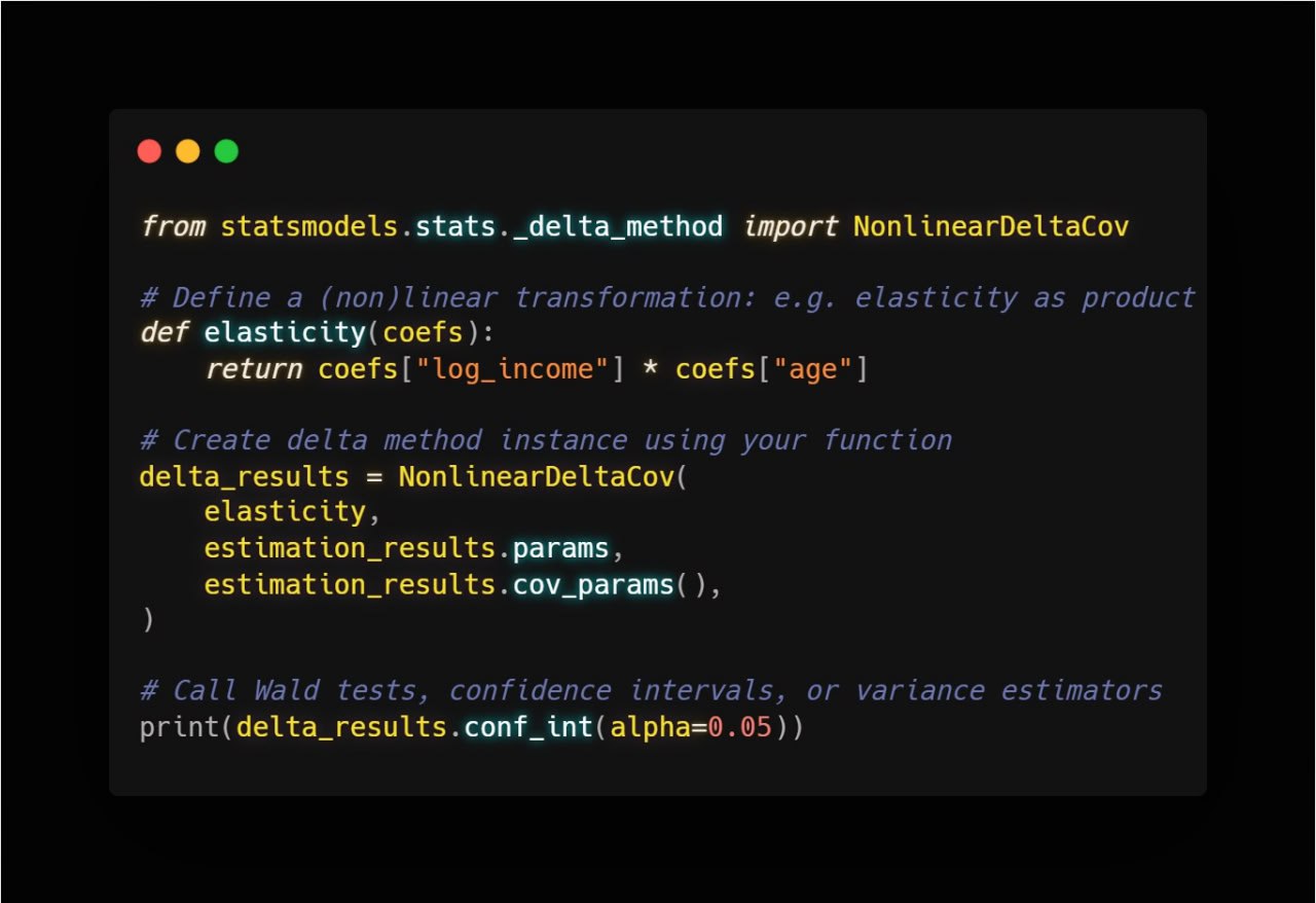
To apply this to our parameter of interest, we create an instance of NonlinearDeltaCov using three key arguments:
- The function \(f(\cdot)\) of interest, which takes the estimates as an argument.
- The estimated parameters.
- The estimated asymptotic variance matrix of the estimator.
In our example, we can create an instance of NonlinearDeltaCov by accessing the params and the cov_params() of the results object:
delta_ratio = NonlinearDeltaCov(
    max_earn,
    results.params,
    results.cov_params()
)
It’s worth noting that while we’ve used an OLS instance here, NonlinearDeltaCov is compatible with any estimation approach that provides parameter estimates and a suitable estimated asymptotic covariance matrix.
We can now look at three basic methods of NonlinearDeltaCov that cover most practical applications:
- A summary method. It prints a basic summary: estimated value, standard error, \(t\)-statistics, and confidence interval:
delta_ratio.summary(alpha=0.05)
                            Test for Constraints
==============================================================================
                coef    std err          z      P>|z|      [0.025      0.975]
------------------------------------------------------------------------------
c0            32.8910      1.287     25.550      0.000      30.368      35.414
==============================================================================
(Note: the printed title refers to “Test for Constraints”, likely a leftover from another use case.)
- A confidence interval method. If just a confidence interval is necessary, easy to construct one with
conf_int()method
delta_ratio.conf_int(alpha=0.05)
array([[30.36791181, 35.41407441]])
- A Wald test method. Suppose that we wish to test that earnings are maximized after 15 years of work:
The wald_test() method works like other tests in statsmodels
delta_ratio.wald_test(np.array([15]))
(np.float64(193.1535027123987), np.float64(6.516561763470986e-44))
The results indicate a strong rejection of the null hypothesis, suggesting that the earnings peak is significantly different from 15 years of work.