Why Adding Fixed Effects May Increase Bias

Posted in Statistics / Heterogeneity

Why adding (more) fixed effects is not a silver bullet for the problem of unobserved heterogeneity and 3 things you can do about it.

A common approach to controlling for unobserved heterogeneity is to run a linear regression with fixed effects. This post shows that this strategy may lead to strong bias in more realistic settings, even if you specify the fixed effects correctly. It is also about some things you can do about it.

• Introduction: the Problem
  • The Setting
  • The Problem with Fixed Effects and This Post
• A Simulation Study: the Issues of the FE Estimator
  • Setting and Estimators Compared
  • Results: Distribution of Estimators
  • Takeaway: Do Not Trust Estimate Changes after Adding Fixed Effects
• When the FE Estimators Is Usable (and When Not)
  • Conditions for Consistency of the FE Estimator
  • A Sufficient Condition for \(\mathbb{E}[\tilde{\boldsymbol{X}}_i'\tilde{\boldsymbol{X}}_i\boldsymbol{\eta}_i]=0\)
  • \(\mathbb{E}[\tilde{\boldsymbol{X}}_i'\tilde{\boldsymbol{X}}_i\boldsymbol{\eta}_i]\) and Adding More Effects
• Practical Advice and Conclusions
  • Solution 1: An Honest Approach to the FE Estimator
  • Solution 2: A Robust Approach with the Mean Group Estimator
  • Solution 3: A Robust Approach with Grouped Estimation
  • Conclusions
• References

If math is messed up, reload the page so that MathJax has another go.

Introduction: the Problem

The Setting

Suppose that we want to estimate the average effect of some variables \(\boldsymbol{x}\) on some outcome \(y\). For example, \(\boldsymbol{x}\) can be investment in R&D by a firm, and \(y\) can be worker productivity. In another example, \(\boldsymbol{x}\) can be air pollution on a given day, and \(y\) can be the crime rate on that day.

By now everyone agrees that you have to do something about unobserved heterogeneity — there is a lot of unobserved differences between units in any economic and business data. Firms differ in their technology, culture, and managerial capacity, etc. Consumers differ in their preferences, social ties, and expectations; etc.

Common approach: adding fixed effects A common solution is to obtain panel data and run a linear regression with “fixed effects” (FEs):

\(\hspace{1cm} y_{it} = \alpha_i + (\text{other fixed effects}_{it}) + \boldsymbol{\beta}' \boldsymbol{x}_{it} + u_{it}, \quad i=1,\dots, N, \quad t=1, \dots, T \qquad (1)\)

The fixed effects are just heterogeneous constants. The simplest kind are the unit-level effects \(\alpha_i\). Other effects can include time-specific intercepts \(\delta_t\) (two-way FEs), or some more complex combinations, such as industry \(\times\) year interacted FEs.

The hope is that you will “control” for unobserved heterogeneity if you add “enough” FEs. In this case, \(\boldsymbol{\beta}\) should capture the effect of \(\boldsymbol{x}\) on \(y\). \(\boldsymbol{\beta}\) can be estimated by eliminating the FEs from Equation 1 and estimating the resulting equation — an approach known as FE (or within) estimation.

The Problem with Fixed Effects and This Post

But why homogeneous \(\boldsymbol{\beta}\)? A key problem with Equation 1 is that it is not an internally consistent model. Why should the slopes \(\boldsymbol{\beta}\) be the same for all units? This assumption goes against acknowledging heterogeneity and including FEs. Would it not be reasonable to specify the more flexible model where the slopes can also be heterogeneous:

\(\hspace{1cm} y_{it} = \alpha_i + (\text{other fixed effects}_{it}) + \color{red}{\boldsymbol{\beta}_i}' \boldsymbol{x}_{it} + u_{it}, \quad i=1,\dots, N, \quad t=1, \dots, T \qquad(2)\)

I personally struggle to think of a single convincing example where the \(\boldsymbol{\beta}\) are homogeneous, while the constant terms can be heterogeneous.

What is this post about? Problems with FEs and Solutions In this post, I show that the strategy of using FEs breaks down under the more realistic Equation 2 and discuss some solutions. Specifically, we will see that:

1. The FE estimator may be catastrophically biased even if you correctly specify the FEs.

2. If you add additional fixed effects, you may increase bias in estimation and get worse results than if you didn’t do anything about heterogeneity.

3. There is a precise condition on the data under which the FE estimator does correctly estimate the average effects.

4. Some solutions are available: ranging from simply explicitly thinking about the assumptions needed for consistent estimation to using estimators robust to parameter heterogeneity.

The full simulation code is available on the blog codes repository.

The issues with the fixed effects estimators are well-known at least in the case of two-way effects in diff-in-diff settings (De Chaisemartin and D’Haultfœuille 2020). This post argues that the problems with FE estimators are much more general: the appear in all contexts, no just diff-in-diff, and affect any configuration of fixed effects.

A Simulation Study: the Issues of the FE Estimator

Setting and Estimators Compared

Let us start with the problems. It is easiest to show the issue with a small simulation study.

Outcome equation Suppose that the outcome \(y_{it}\) is generated with a very simple model which only has one individual fixed effect \(\alpha_i\) and only two periods of data: \[y_{it} = \alpha_i + (\beta + \alpha_i) x_{it} + u_{it}, \quad i=1, \dots, N, \quad t=1, 2, \quad \mathbb{E}[u_{it}| x_{i1}, x_{i2}] =0,\]

where \(\beta\) is the parameter of interest — the average coefficient vector (average effect). We set \(\beta\) to be negative: \[\beta = - 0.25.\]

There are only two types of units in terms \(\alpha_i\): \(\alpha_i\) is equal to \(+1\) and \(-1\) with equal probabilities. Accordingly, half the units in population have a positive slope of \(0.75\), and half have a negative slope of \(-1.25\).

Estimators compared: FE vs. no FE We compare two estimators for \(\beta\):

1. Simple pooled OLS regression (no fixed effects), which involves estimating the model \[y_{it} = \beta x_{it} + w_{it}, \quad\quad\quad w_{it} = \alpha_i + \alpha_i x_{it} + u_{it}\]

2. The fixed-effects/within estimator that correctly specifies the unit-level random intercepts. In this case we estimate the following model: \[y_{it} = \alpha_i + \beta x_{it} + v_{it}, \quad\quad\quad v_{it} = \alpha_i x_{it} + u_{it}.\]

While just these two estimators are sufficient to illustrate the point, it is straightforward to consider designs with more random intercepts — time effects, interacted effects, different groupings, etc.

The rest of the DGP The rest of the data-generating process (DGPs) is such that the pooled OLS estimator is unbiased, while the FE estimator is biased. See the fold-out for details.

Details of the GDP

The rest of the DGP is specified as follows:

1. Conditional on a given value of \(\alpha_i, (x_{i1}, x_{i2})\) is bivariate normal with parameters that depend on whether \(\alpha_i = +1\) or \(\alpha_i = -1\): \[\begin{pmatrix} x_{i1} \\ x_{i2} \end{pmatrix}\Bigg| \alpha_i = + 1 \sim N\left( \begin{pmatrix} \mu_{1+} \\ \mu_{2+} \end{pmatrix}, \begin{pmatrix} \sigma_{1+}^2 & \rho_+ \sigma_{1+} \sigma_{2+} \\ \rho_+ \sigma_{1+} \sigma_{2+} & \sigma_{2+}^2 \end{pmatrix} \right)\]

   and \[\begin{pmatrix} x_{i1} \\ x_{i2} \end{pmatrix}\Bigg| \alpha_i = - 1 \sim N\left( \begin{pmatrix} \mu_{1-} \\ \mu_{2-} \end{pmatrix}, \begin{pmatrix} \sigma_{1-}^2 & \rho_- \sigma_{1-} \sigma_{2-} \\ \rho_- \sigma_{1-} \sigma_{2-} & \sigma_{2-}^2 \end{pmatrix} \right).\]

2. \(u_{it}\) is standard normal and independent of the other components in the model.

We set the parameters for the distribution of \(x_{it}\) so that the OLS estimator is consistent and the FE estimator is inconsistent. Specifically, we select the parameters so that the following conditions are satisfied: \[\begin{aligned} \mathbb{E}[x_{it}(\alpha_i + \alpha_i x_{it}+ u_{it})] & = 0, \quad t=1, 2, \\ \mathbb{E}[(x_{i2}- x_{i1})(\alpha_i (x_{i2}- x_{i1})+ u_{it})] & \neq 0 . \end{aligned}\]

Note that \((x_{i2}-x_{i1})\) is exactly the within-transformed regressor involved in the FE regression.

We find some parameters by simply specifying a nonzero value for the second expectations and searching for a root of the resulting equations — simply applying GMM in population.

Here is a simple Python implementation of a GMM solver class:

import numpy as np

from scipy.optimize import minimize
from typing import Callable, List, Dict, Any, Optional

class GMMSolver:
    """
    A Generalized Method of Moments (GMM) solver that estimates parameters by 
    minimizing the weighted squared distance of moment conditions from zero.

    Attributes:
        moment_conditions (Callable[[np.ndarray], np.ndarray]):
            Function returning moment conditions given parameter values.
        constraints (Optional[List[Dict[str, Any]]]):
            List of constraints for parameter optimization.
        initial_guess (np.ndarray):
            Initial parameter values for the optimization.
        weighting_matrix (np.ndarray):
            Weighting matrix for the GMM objective function. Defaults to identity.
        process_func (Callable[[np.ndarray], Dict[str, Any]]):
            Function that processes the optimized parameters into a meaningful format.
    """

    def __init__(
        self,
        moment_conditions: Callable[[np.ndarray], np.ndarray],
        initial_guess: np.ndarray,
        constraints: Optional[List[Dict[str, Any]]] = None,
        weighting_matrix: Optional[np.ndarray] = None,
        process_func: Optional[Callable[[np.ndarray], Dict[str, Any]]] = None
    ) -> None:
        """
        Initializes the GMM solver with the moment conditions and optimization settings.

        Args:
            moment_conditions (Callable[[np.ndarray], np.ndarray]):
                A function that takes a parameter vector and returns moment conditions.
            initial_guess (np.ndarray):
                Initial parameter values for optimization.
            constraints (Optional[List[Dict[str, Any]]], optional):
                Constraints for optimization. Defaults to None.
            weighting_matrix (Optional[np.ndarray], optional):
                Weighting matrix for GMM. Defaults to identity matrix.
            process_func (Optional[Callable[[np.ndarray], Dict[str, Any]]], optional):
                Function to format the final parameter estimates. Defaults to None.
        """
        self.moment_conditions = moment_conditions
        self.initial_guess = np.array(initial_guess)
        self.constraints = constraints if constraints else []
        self.weighting_matrix = (
            np.eye(len(moment_conditions(initial_guess))) if weighting_matrix is None else weighting_matrix
        )
        self.process_func = process_func
        self.estimated_params = None

    def _gmm_objective(self, params: np.ndarray) -> float:
        """
        Computes the GMM objective function: 
        m(θ)ᵀ W m(θ), where m(θ) are the moment conditions.

        Args:
            params (np.ndarray): Current parameter estimates.

        Returns:
            float: The GMM loss function value.
        """
        moments = self.moment_conditions(params) 
        return moments.T @ self.weighting_matrix @ moments

    def minimize(self) -> None:
        """
        Runs the GMM estimation by minimizing the GMM objective function.

        Returns:
            np.ndarray: The estimated parameters.
        """
        result = minimize(self._gmm_objective, self.initial_guess, constraints=self.constraints)

        if not result.success:
            raise ValueError(f"Optimization failed: {result.message}")

        self.estimated_params = result.x

    def process_solution(self) -> Dict[str, Any]:
        """
        Processes the estimated parameters into a meaningful format.

        Returns:
            Dict[str, Any]: Processed output, depends on user-supplied processing function.
        """
        if self.process_func is None:
            return {"parameters": self.estimated_params}
        return self.process_func(self.estimated_params)

The moments, constraints, and processing functions are defined as follows

def sim_moment_conditions(params: np.ndarray) -> np.ndarray:
    """ 
    Moment conditions for consistency of OLS and inconsistency of FE estimators.

    Args:
        params (np.ndarray): Parameter values.

    Returns:
        np.ndarray: Moment equations evaluated at given parameters.
    """
    sigma1p, sigma2p, rhop, mu1p, mu2p, sigma1m, sigma2m, rhom, mu1m, mu2m = params

    return np.array([
        sigma2p**2 + mu2p**2 + mu2p - sigma2m**2 - mu2m**2 - mu2m,
        sigma1p**2 + mu1p**2 + mu1p - sigma1m**2 - mu1m**2 - mu1m,
        sigma1p**2 + sigma2p**2 - 2 * rhop * sigma1p * sigma2p 
        + mu2p**2 + mu1p**2 - 2 * mu1p * mu2p
        - sigma1m**2 - sigma2m**2 + 2 * rhom * sigma1m * sigma2m
        - mu2m**2 - mu1m**2 + 2 * mu1m * mu2m
        - 1000
    ])

def process_mu_sigma_params(params: np.ndarray) -> dict:
    """
    Extracts mu and sigma matrices from the parameters vector.

    Args:
        params (np.ndarray): Estimated parameter values.

    Returns:
        dict: Processed parameters (mu and sigma matrices).
    """
    mu_plus = params[3:5]
    mu_minus = params[8:]

    sigma_plus = np.array([
        [params[0]**2, (params[0] * params[1]) * params[2]],
        [(params[0] * params[1]) * params[2], params[1]**2]
    ])
    sigma_minus = np.array([
        [params[5]**2, (params[5] * params[6]) * params[7]],
        [(params[5] * params[6]) * params[7], params[6]**2]
    ])

    return {"mu_plus": mu_plus, 
            "mu_minus": mu_minus, 
            "sigma_plus": sigma_plus, 
            "sigma_minus": sigma_minus,
            }

# Constraints on data-generating process parameters
constraints = [
    {'type': 'ineq', 'fun': lambda vars: vars[0]},  # sigma_{1+} >= 0
    {'type': 'ineq', 'fun': lambda vars: vars[1]},  # sigma_{2+} >= 0
    {'type': 'ineq', 'fun': lambda vars: 1 - vars[2]},  # rho_+ <= 1
    {'type': 'ineq', 'fun': lambda vars: vars[2] + 1},  # rho_+ >= -1
    {'type': 'ineq', 'fun': lambda vars: vars[5]},  # sigma_{1-} >= 0
    {'type': 'ineq', 'fun': lambda vars: vars[6]},  # sigma_{2-} >= 0
    {'type': 'ineq', 'fun': lambda vars: 1 - vars[7]},  # rho_- <= 1
    {'type': 'ineq', 'fun': lambda vars: vars[7] + 1},  # rho_- >= -1
]

# Initial guess for parameters
param_initial_guess = [12, 15,  0.3, 24, -7, 2,  8,  0.6,  5, 14]

Finally, we can compute the parameters as:

solver_dgp_params = GMMSolver(
        sim_moment_conditions,
        param_initial_guess,
        constraints, 
        process_func=process_mu_sigma_params,
    )
solver_dgp_params.minimize()
mu_sigma_params = solver_dgp_params.process_solution()
print(mu_sigma_params)

{'mu_plus': array([  1.09064557, -22.60362844]), 
'mu_minus': array([13.7704972 , 25.70151531]), 
'sigma_plus': array([[437.04406675,  64.35128113],
       [ 64.35128113, 440.05540533]]), 
'sigma_minus': array([[235.927077  , 155.28354406],
       [155.28354406, 242.10637242]])}

The values you obtain may differ — there are multiple sets of parameters that yield the desired values for the expectations.

Unfortunately, such a DGP is as plausible as an opposite one where only the FE estimator is consistent. Intuitively, the two cases are equally likely because both involve the same number of restrictions on the parameters (though in this sense both DGPs are less likely than the situation in which both estimators are inconsistent).

As a consequence, one should not dismiss this DGP as an unrealistic edge case.

Results: Distribution of Estimators

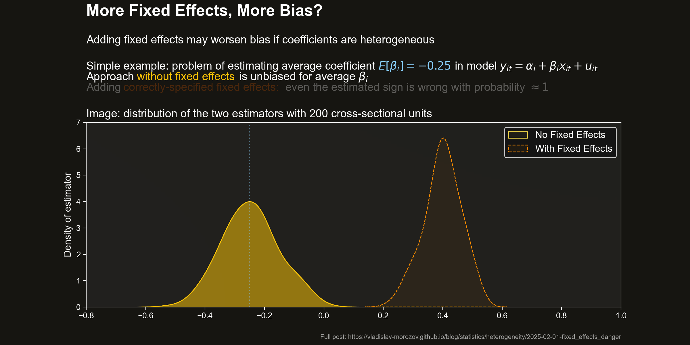
Distribution of estimators Let us take a look at the distribution of the two estimators. The following pictures shows the densities of the estimators for a few values of \(N\). I also highlighted the target value — the average effect \(\beta=0.25\).

Pooled OLS (no fixed effects) does pretty well. It is unbiased and becomes fairly precise even in pretty small sample sizes.

However, adding fixed effects dramatically worsens the situation. The FE estimator is strongly biased. The bias is so large that the target of the FE estimator (a) has a different sign from \(\beta\) and (b) is larger (in absolute value) than the target effect.

Wrong effect sign with FE As a consequence, if you trust the FE estimator, you will with probability \(\approx 1\) conclude that there is a positive effect on average, even for tiny sample sizes:

Takeaway: Do Not Trust Estimate Changes after Adding Fixed Effects

So what does this simulation tell us?

First, the FE estimator can be significantly biased even if the fixed effects themselves are correctly specified. The bias may be so large that not even the sign of the average effect is correctly estimated.

Second, adding FEs may worse estimation quality. The simple example above shows how a smaller model yields estimates preferable to those of a larger model. One should be careful with the false “intuition” that adding more FE better controls for heterogeneity.

When the FE Estimators Is Usable (and When Not)

Is there anything that can be done to estimate the average effect under Equation 2? Several things, as we discuss below. As the first answer, we will consider the conditions under which the FE can yield a consistent estimate for the average effect.

Conditions for Consistency of the FE Estimator

What controls whether the fixed effects estimator is estimating the average effect? Or, put differently, what configurations of fixed effects permit consistent estimation of the average effect with the FE estimator?

Theoretical framework It is straightforward to work out the exact conditions in a fairly general case. Suppose that \(y_{it}\) is generated as \[y_{it} = \text{fixed effects}_{it} + \boldsymbol{\beta}_i' \boldsymbol{x}_{it} + u_{it}, \quad i=1,\dots, N, \quad t=1, \dots, T, \quad \mathbb{E}[u_{it}|\boldsymbol{x}_{i1}, \dots, \boldsymbol{x}_{iT}]=0,\]

where \(\boldsymbol{x}_{it}\) is a vector of covariates. Here \(\text{fixed effects}_{it}\) can stand for one-, two-, or multi-way fixed effects. Any configuration of fixed effects is allowed, as long as it can be eliminated by a suitable within transformation without deleting the full data completely. Let us assume that the residual \(u_{it}\) is strictly exogenous in the sense that \(\mathbb{E}[u_{it}|\boldsymbol{x}_{i1}, \dots, \boldsymbol{x}_{iT}]=0\). This condition rules out dynamic panels where the situation is more complex and the subject of a future post.

Formal definition of the FE estimator Apply the within transformation to eliminate the fixed effects. Label the resulting variables \(\tilde{w}_{it}\) so that the within-transformed variables satisfy \[\tilde{y}_{it} = \boldsymbol{\beta}_i'\tilde{\boldsymbol{x}}_{it} + \tilde{u}_{it}.\]

For each unit \(i\), stack \(\tilde{\boldsymbol{x}}_{it}\) into the matrix \(\tilde{\boldsymbol{X}}_i\). Similarly combine all \(\tilde{y}_{it}\) for a given unit $i$ into the vector \(\tilde{\boldsymbol{y}}_i\). The fixed effect estimator \(\hat{\boldsymbol{\beta}}_{FE}\) can be written as \[\hat{\boldsymbol{\beta}}^{FE} = \left(\sum_{i=1}^N \tilde{\boldsymbol{X}}_i'\tilde{\boldsymbol{X}}_i \right)^{-1} \sum_{i=1}^N \tilde{\boldsymbol{X}}_i \tilde{\boldsymbol{y}}_i.\]

For convenience, define \(\boldsymbol{\eta}_i\) as \[\boldsymbol{\eta}_i = \boldsymbol{\beta}_i - \mathbb{E}[\boldsymbol{\beta}_i] .\]

Characterization of consistency of the FE estimator The following theorem shows that \(\hat{\boldsymbol{\beta}}^{FE}\) consistently estimates \(\mathbb{E}[\boldsymbol{\beta}_i]\) if and only if a particular orthogonality condition holds between the second moments of \(\tilde{\boldsymbol{X}}_i\) and the deviations \(\boldsymbol{\eta}_i\) of the coefficients from their mean.

RESULT: \(\hat{\boldsymbol{\beta}}^{FE}\) converges to \(\mathbb{E}[\boldsymbol{\beta}_i]\) in probability as \(N\to\infty\) if and only if \(\mathbb{E}[\tilde{\boldsymbol{X}}_i'\tilde{\boldsymbol{X}}_i\boldsymbol{\eta}_i] =0.\)

This result first appears in Wooldridge (2003) and Wooldridge (2005).

Proof

Throughout, we assume that all corresponding moments exists and all sample average converge to population averages. We first expand the FE estimator using the within-transformed model: $$ \begin{aligned} \hat{\boldsymbol{\beta}}^{FE} & = \left(\sum_{i=1}^N \tilde{\boldsymbol{X}}_i'\tilde{\boldsymbol{X}}_i \right)^{-1} \sum_{i=1}^N \tilde{\boldsymbol{X}}_i \tilde{\boldsymbol{y}}_i \\ & = \left(\sum_{i=1}^N \tilde{\boldsymbol{X}}_i'\tilde{\boldsymbol{X}}_i \right)^{-1} \sum_{i=1}^N \tilde{\boldsymbol{X}}_i \tilde{\boldsymbol{X}}_i\boldsymbol{\beta}_i + \left(\sum_{i=1}^N \tilde{\boldsymbol{X}}_i'\tilde{\boldsymbol{X}}_i \right)^{-1} \sum_{i=1}^N \tilde{\boldsymbol{X}}_i \tilde{\boldsymbol{u}}_i. \end{aligned} $$ Substituting the definition of the deviations from the average coefficients nets us $$ \begin{aligned} \hat{\boldsymbol{\beta}} & = \mathbb{E}[\boldsymbol{\beta}_i] + \left( \dfrac{1}{N}\sum_{i=1}^N \tilde{\boldsymbol{X}}_i'\tilde{\boldsymbol{X}}_i \right)^{-1} \dfrac{1}{N}\sum_{i=1}^N \tilde{\boldsymbol{X}}_i \tilde{\boldsymbol{X}}_i\boldsymbol{\eta}_i + \left( \dfrac{1}{N}\sum_{i=1}^N \tilde{\boldsymbol{X}}_i'\tilde{\boldsymbol{X}}_i \right)^{-1} \dfrac{1}{N}\sum_{i=1}^N \tilde{\boldsymbol{X}}_i \tilde{\boldsymbol{u}}_i\\ & \xrightarrow{p} \mathbb{E}[\boldsymbol{\beta}_i] + \left(\mathbb{E}\left[\tilde{\boldsymbol{X}}_i'\tilde{\boldsymbol{X}}_i \right] \right)^{-1} \mathbb{E}\left[\tilde{\boldsymbol{X}}_i'\tilde{\boldsymbol{X}}_i\boldsymbol{\eta}_i \right] + \left(\mathbb{E}\left[\tilde{\boldsymbol{X}}_i'\tilde{\boldsymbol{X}}_i \right] \right)^{-1} \mathbb{E}\left[\tilde{\boldsymbol{X}}_i'\tilde{u}_i \right]\\ & = \mathbb{E}[\boldsymbol{\beta}_i] + \left(\mathbb{E}\left[\tilde{\boldsymbol{X}}_i'\tilde{\boldsymbol{X}}_i \right] \right)^{-1} \mathbb{E}\left[\tilde{\boldsymbol{X}}_i'\tilde{\boldsymbol{X}}_i\boldsymbol{\eta}_i \right]. \end{aligned} $$ The result can now be read off from the last display.

A Sufficient Condition for \(\mathbb{E}[\tilde{\boldsymbol{X}}_i'\tilde{\boldsymbol{X}}_i\boldsymbol{\eta}_i]=0\)

It is not obvious when \(\mathbb{E}[\tilde{\boldsymbol{X}}_i'\tilde{\boldsymbol{X}}_i\boldsymbol{\eta}_i]=0\). To me, it is usually not even clear what it means — the condition involves \(\boldsymbol{\eta}_i\) and the second moments of the within-transformed covariates.

Strong sufficient condition: full independence The condition will certainly hold if \(\boldsymbol{\beta}_i\) and \(\boldsymbol{X}_i\) are independent. However, you only really expect this independence in marginally randomized experiments. It is extremely unlikely to hold in observational data.

More general sufficient condition: mean independence Luckily, there is a simple sufficient condition that does not require full independence. It is sufficient that \(\boldsymbol{\eta}_i\) is mean-independent from \(\tilde{\boldsymbol{X}}\) in the following sense: \[\mathbb{E}[\boldsymbol{\eta}_i|\tilde{\boldsymbol{X}}_i] = 0.\]

Intuition: case of unit-level FEs To get some intuition, consider the simplest case where only individual-level effects are present: \[y_{it} = \alpha_i + \boldsymbol{\beta}_i'\boldsymbol{x}_{it} + u_{it}.\]

In this case, the within transformation simply subtracts individual time averages, that is, \[\tilde{\boldsymbol{x}}_{it} = \boldsymbol{x}_{it} - \dfrac{1}{T} \sum_{t=1}^T \boldsymbol{x}_{it}.\]

The within transformation removes permanent (=static) components in \(\boldsymbol{x}_{it}\). What is left are the dynamics in \(\boldsymbol{x}_{it}\). Accordingly, the above condition requires that the changes in \(\boldsymbol{x}_{it}\) over time are not informative about the individual coefficients.

\(\mathbb{E}[\tilde{\boldsymbol{X}}_i'\tilde{\boldsymbol{X}}_i\boldsymbol{\eta}_i]\) and Adding More Effects

Can we say anything about how \(\mathbb{E}[\tilde{\boldsymbol{X}}_i'\tilde{\boldsymbol{X}}_i\boldsymbol{\eta}_i]\) or \(\mathbb{E}[\boldsymbol{\eta}_i|\tilde{\boldsymbol{X}}_i]\) as we add more fixed effects?

Unfortunately, very little can be said in general. Adding more FEs changes the definition of \(\tilde{\boldsymbol{X}}_i\) and reduces the remaining variation in the covariates. In principle, this reduction makes it easier for the condition \(\mathbb{E}[\boldsymbol{\eta}_i|\tilde{\boldsymbol{X}}_i]=0\) to be satisfied, since the expectation conditions on progressively less information. In the limit the fixed effects are rich enough so that \(\tilde{\boldsymbol{X}}_i=\varnothing\), and then automatically \(\mathbb{E}[\boldsymbol{\eta}_i|\tilde{\boldsymbol{X}}_i]=\mathbb{E}[\boldsymbol{\eta}_i]=0\). However, at this point there is no variation left in the covariate, so no estimation is possible.

It is also generally impossible to predict the direction of change in \(\mathbb{E}[\tilde{\boldsymbol{X}}_i'\tilde{\boldsymbol{X}}_i\boldsymbol{\eta}_i]\) as an additional layer of FEs is added. Such an addition may either bring \(\mathbb{E}[\tilde{\boldsymbol{X}}_i'\tilde{\boldsymbol{X}}_i\boldsymbol{\eta}_i]\) closer to zero, or push it further away, as in the simulation.

Practical Advice and Conclusions

So what should one do in practice? Ignoring the issue seems unreasonable and internally inconsistent, as pointed out in the introduction.

However, there are (at least) three solutions which seem reasonable to me.

Solution 1: An Honest Approach to the FE Estimator

The minimal solution is to at least acknowledge that the FE estimator is only consistent under the condition that \(\mathbb{E}[\tilde{\boldsymbol{X}}_i'\tilde{\boldsymbol{X}}_i\boldsymbol{\eta}_i]=0\) (or some other version of this condition appropriate to the assumed pattern of heterogeneity in the coefficients). If you wish to trust the FE estimator, you should first justify why the above condition holds in your particular empirical setting.

Solution 2: A Robust Approach with the Mean Group Estimator

A more ambitious solution is to use a heterogeneity-robust approach — the mean group estimator (Pesaran and Smith 1995) or one of its refinements (Breitung and Salish 2021). This approach has a data price — \(T\) must be larger than the number of covariates. If this condition is satisfied and there is enough variation in the individual data, one can then run unit-by-unit regressions. The mean group estimator is simply the cross-sectional average of these individual estimators. It is not hard to show that it is consistent for \(\mathbb{E}[\boldsymbol{\beta}_i]\) without any assumptions on how \(\boldsymbol{\beta}_i\) and \(\boldsymbol{X}_i\) are related.

Solution 3: A Robust Approach with Grouped Estimation

A different flexible approach is to try grouped estimators in the style of Bonhomme and Manresa (2015). This approach is more appropriate if \(T\) is large and one is unwilling to believe that the coefficients \(\beta_i\) are invariant in the data.

Conclusions

In summary, one should not consider the strategy of specifying fixed effects as a sufficient way of controlling for heterogeneity. Under parameter heterogeneity, the FE estimator may in general be quite biased even if the FEs are specified correctly. To solve this issue, one should either think carefully about the empirical setting or use heterogeneity-robust approaches.

References

1. Bonhomme, Stéphane, and Elena Manresa. 2015. “Grouped Patterns of Heterogeneity in Panel Data.” Econometrica 83 (3): 1147–84. https://doi.org/10.3982/ecta11319.
2. Breitung, Jörg, and Nazarii Salish. 2021. “Estimation of Heterogeneous Panels with Systematic Slope Variations.” Journal of Econometrics 220 (2): 399–415.https://doi.org/10.1016/j.jeconom.2020.04.007.
3. De Chaisemartin, Clément, and Xavier D’Haultfœuille. 2020. “Two-Way Fixed Effects Estimators with Heterogeneous Treatment Effects.” American Economic Review 110 (9): 2964–96. https://doi.org/10.1257/aer.20181169.
4. Pesaran, M. Hashem, and Ron P. Smith. 1995. “Estimating long-run relationships from dynamic heterogeneous panels.” Journal of Econometrics 6061: 473–77.
5. Wooldridge, Jeffrey M. 2003. “Fixed Effects Estimation of the Population-Averaged Slopes in a Panel Data Random Coefficient Model.” Econometric Theory 19: 411–13. https://doi.org/10+10170S0266466603002081.
6. ———. 2005. “Fixed-effects and related estimators for correlated random-coefficient and treatment-effect panel data models.” The Review of Economics and Statistics 87 (May): 385–90.